
From Prompt to Power
A Survey of Models, Chips, and Infrastructure
This course is for anyone with basic in computer science who wants to understand how modern works and what has to happen across its supply chain. No background in machine learning or chip design is required. Concepts are introduced in ordinary language as they appear, so readers without a technical background should still be able to follow most of the course.
The central idea is simple: an product is not only a . Every answer depends on a chain of software, chips, , networking, centers, electricity, manufacturing, and money. A limit or delay anywhere in that chain can affect what the user experiences and what the service costs.
An answer from artificial intelligence, or , may feel weightless, but physical machines make it. An is a learned system of calculations that turns an input into a prediction or other output. A is one built to and generate language at a scale; it can contain billions of learned . Running it moves through , performs , and uses electricity. Those physical limits affect speed and cost.
This course follows that chain from the user outward:
your request
    -> a model predicts an answer
    -> chips move data and do arithmetic
    -> data centers supply power, cooling, and connections
    -> someone pays for every second of the process
A chip specification means little until you know the job the chip must do. A price per chip-hour means little until you know how many useful answers that hour produces. Part 0 introduces the units used throughout. The rest of the course follows a compact map:
- Workloads, Parts 1–3: , , and .
- The machine, Parts 4–9: why graphics processors work, what is inside them, , , manufacturing, and connections.
- Decisions, Parts 10–11: choosing hardware and understanding economics.
performance is never one . A system can have fast and slow , cheap chips and expensive power, or an impressive maximum speed that useful work never reaches. For repeated work, the most constrained required resource often limits how much the system finishes per second; several stages may still add to the delay of one request.
How facts are handled. Real product, , and market are sourced, and volatile figures are dated. Examples introduced with “suppose” are illustrative , not market quotes. Claims that cannot be supported or usefully qualified are omitted.
Part 0 — A Small Vocabulary for Big Systems
This opening introduces four quantities used throughout the course: , stored and moved , power and energy, and . Keep each amount separate from its rate.
0.1 Work Is Different From Speed
A job has a fixed amount of work, while a machine has a rate at which it can attempt that work. Confusing the two is like confusing miles with miles per hour.
Many calculations multiply and add that can represent fractions. Engineers count those individual steps as , or . Under the convention used in most hardware specifications, one addition or one multiplication is one operation. A combined multiply-and-add is two because it performs both steps. A rate can be written /s, meaning per second. Because the abbreviations for an amount and a rate are easy to confuse, this course usually writes “operations” and “operations per second” in full.
Suppose a job needs 1,000 operations and a processor actually completes 100 operations each second. The alone takes 10 seconds:
time = amount of work ÷ achieved rate
     = 1,000 operations ÷ 100 operations per second
     = 10 seconds
The word achieved matters. A specification normally gives the highest rate the hardware can reach for a particular kind of and operation. A real program may spend part of its waiting for , another processor, or a result on which its next step depends. A peak operations-per-second figure is therefore a ceiling under stated conditions, not a promise that every program will run at that speed.
0.2 Stored Data Is Different From Moved Data
asks how much fits. asks how much can pass a named point each second. A warehouse can hold a million boxes and still have one narrow loading door. The first fact describes capacity; the second describes .
Suppose a machine must read a 100 GB file from and can sustain 50 GB per second. The transfer takes at least two seconds if nothing else uses that path. Doubling the capacity of the would let the machine hold more files, but it would not make this transfer faster. Doubling the could reduce the transfer , but it would not create room for a larger file. Later Parts apply this distinction to : the must fit before their delivery speed matters.
A represents one of two values, conventionally zero or one. Eight make one . In decimal units, one gigabyte (GB) is exactly one billion ; 2³⁰ is one gibibyte (GiB). A quoted of 100 GB per second means 100 billion per second, but the label must say whether that rate is a theoretical maximum or a measurement. Network specifications often count rather than . Dividing by eight converts the units to ; the extra information needed to format and deliver network can make the useful rate lower. NIST defines decimal and binary data units here.
0.3 Power Is Different From Energy
tells you how quickly a device is using energy at a moment in . It is measured in watts. tells you how much was used over a period of . Electricity bills normally charge for energy in kilowatt-hours.
Follow one server through an hour. Suppose it draws one kilowatt while a job runs:
energy = power × time
       = 1 kilowatt × 1 hour
       = 1 kilowatt-hour

electricity cost = 1 kilowatt-hour × $0.10 per kilowatt-hour
                 = $0.10
If the same server runs for 10 hours at the same power, it uses 10 kilowatt-hours. Its power did not become “10 kilowatts”; the device drew one kilowatt for longer. Likewise, a device rated at one kilowatt does not necessarily draw that amount at every moment.
The server is not the whole facility. Fans, pumps, power-conversion equipment, networking, and other support systems also use electricity. When someone quotes a power or energy figure, ask three questions: Is it a maximum or a measurement? Over what period? Does it describe one chip, one server, one rack, or the entire center?
0.4 Models Consume and Produce Tokens
Language do not receive text as words on a page. A first divides the text into pieces called and assigns an integer identifier to each piece. A might be a whole common word, part of a less common word, punctuation, or even a space joined to nearby text. The exact pieces come from that 's and rules.
For intuition, imagine that a divides “unbelievable!” into un, believ, able, and !. Those are illustrative pieces, not a claim about a particular . The receives the corresponding identifiers and later produces identifiers that the service converts back into text. Two can divide the same sentence differently, so a word count cannot determine an exact count.
For OpenAI , a useful English-only guide is about three-quarters of a word per . The ratio changes with the language, text, , and . OpenAI explains this estimate and its limits.
A also contains learned values called . Many are numerical that control how strongly one set of affects another; can include other learned adjustments too. A “70-billion- ” contains about 70 billion learned values under its publisher's counting convention. Those values are not 70 billion sentences or database entries. They work together inside the 's calculations.
describe the input and output length. describe the size of the 's learned state. A request with more usually requires more work even though the count stays fixed. A with more usually needs more storage and when its design and are otherwise comparable. Neither , by itself, measures answer quality.
Carry two habits : attach “per what?” to every rate, and ask whether a figure is a theoretical maximum or a measured result.
Part 1 — Inference: How an Answer Gets Made
Most chat-oriented language generate text by selecting a next , adding it to the sequence, and repeating. They do not normally prepare the complete answer in one pass. This explains streaming text and part of the cost of long conversations. Serving requests together can reduce cost, but does not guarantee it. Using a trained to produce an output is called .
1.1 From Pressing Enter to Seeing Text
Pressing Enter does not send words straight into a and receive a finished paragraph back. A service first prepares the request, then the predicts one output at a . The whole journey has five stages:
- Route the request. A web service may check who is calling, enforce its rules, and send the request to a machine that can access the .
- Assemble the input. The service selects instructions, earlier messages, retrieved material, results, and the new message. That history is logically part of the current call even when a service part of it; the does not keep human-like memories between independent calls.
- Turn text into numbered pieces. A divides text according to its and rules, then maps each to an integer identifier. Vocabularies and splitting rules differ among families. This conversion is called .
- the input and select the first answer piece. The produces a numerical score for each in its , and a decoding rule uses those scores to select the next . It might select “Rise” rather than “Sourdough” in response to “Name my bakery.” Processing the and preparing reusable is called .
- Build the rest one piece at a . In ordinary , the selected becomes part of the sequence and the runs another step. This answer-building phase is called . Generation can stop at an end , a configured limit, or another stopping rule. The service then turns identifiers into readable text.
Input:  Name a bakery that sells only sourdough.

Read the full input             -> “Rise”
Read the input plus “Rise”      -> “and”
Read the input plus “Rise and”  -> “Loaf”
Read through “Rise and Loaf”    -> ending marker

Output: Rise and Loaf
Because each accepted output depends on those before it, ordinary answer generation proceeds in order. This creates two phases of serving, explained next.
1.2 The First-Token Pause and the Typing Phase
The pause before an answer and the spacing between later are two different delays. A service can improve one without improving the other, so a single “speed” can hide what the user will feel.
click Send                 first token                  last token
    |--------------------------|---|---|---|---|---|--------|
       time to first token        gaps between output tokens
The first span can include network travel, waiting for a machine, preparing the request, processing the , and selecting the first . The smaller later spans show the pace of ordinary answer generation.
During , the processes the together, so much of the work can run in parallel. Longer usually require more work. is the elapsed from submitting a request until receiving the first output ; it can include network travel, waiting, text conversion, request setup, and . NVIDIA defines this measurement boundary in its inference metrics guide.
During ordinary , output are committed in order, and each step uses the 's learned again. The elapsed between output is , which appears as typing speed to the user.
Why can a chip with enormous capacity still generate slowly? For one or a few requests, each generation step may have to fetch most of the 's from and use them only once. Fetching those can take longer than doing the . The limit is : how many can supply each second. This pattern is common, not universal.
Consider a deliberately optimistic one-user example. Suppose such a 's occupy 70 GB and an —a processor built to perform calculations efficiently—has a peak of 3,350 GB per second. If each step must stream those once, traffic alone gives an upper bound of 3,350 ÷ 70, or about 48 steps—and therefore about 48 output —per second. Real is lower when the peak is not sustained and because reads, temporary values, synchronization, and other work also consume and . The figure matches NVIDIA's published peak for one H100 server-module configuration, not a measured application result. NVIDIA H100 specifications, accessed July 2026.
The meaning of the estimate matters more than the exact figure. On a specified machine, work limited mainly by is ; work limited mainly by traffic is . Long or well-batched can be , while generating for only a few requests is often . length, design, of simultaneous requests, software, and hardware can change the result.
1.3 How a Transformer Uses the KV Cache
The main idea is simple: a predicts one next , adds the selected to the sequence, and repeats. To make each repeat less wasteful, serving software keeps some that the already calculated for earlier . Those saved form the , or .
The is not a written summary of the conversation, and it does not make the prediction by itself. The still runs every for each new . The merely prevents those layers from rebuilding the same key and value for all earlier . Each new must still compare with and read the saved . This is why the saves while also consuming and . Hugging Face's implementation guide shows the cache being updated and read separately in every attention layer.
First, follow one next-token prediction
Consider this :
The musician tuned the piano before the concert. Then she played the
Suppose the selects piano as the next . That outcome is plausible, not guaranteed. To keep the example readable, the words are shown as if each were one ; a real may divide the text differently. The reaches its selection in six broad steps:
- Turn each into . The 's identifier selects an : a learned list of that gives the a numerical starting representation for that . The also represents where the occurs in the sequence; designs differ in how they supply that position information to .
- Let positions exchange information. An calculation allows each position to combine information from itself and earlier positions. It cannot use later positions that have not been generated. In the example, the representation at the final the can be influenced by earlier positions such as musician, tuned, and piano.
- Refine each position separately. A applies another learned calculation to each position. moves information among positions; this block transforms the information now held at each position.
- Repeat those two kinds of work. One block followed by one makes up the simplified core of a . A passes the representations through many such layers, so later layers work with information already shaped by earlier layers.
- Score every allowed output . After the final layer, the representation at the last position is mapped to one score for every in the 's . Those scores are converted into probabilities.
- Select and append one . A decoding rule selects a , perhaps piano, and appends it to the sequence. The then runs again to predict what follows piano.
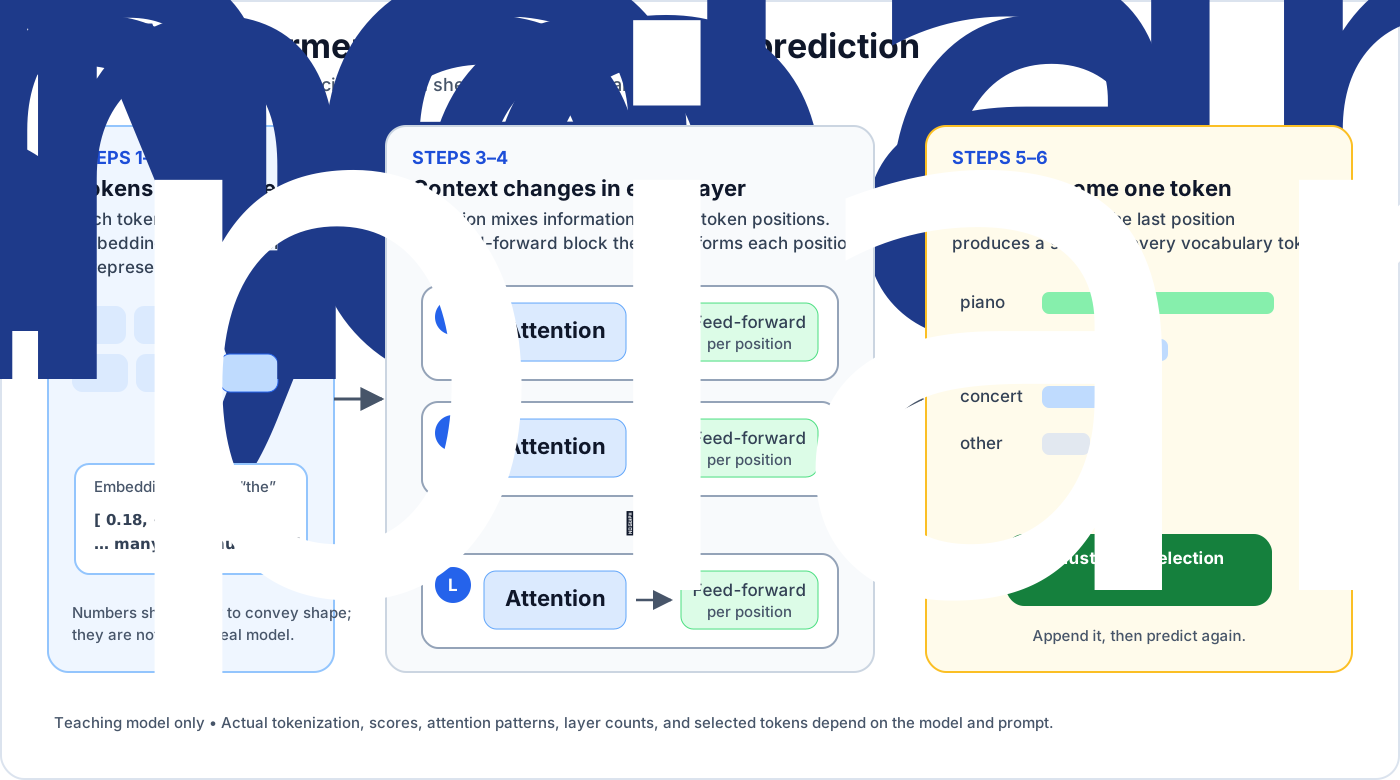
This teaching sequence follows the visual route in 3Blue1Brown's transformer explainer: become numerical representations, and calculations repeatedly change those representations, the final representation becomes scores, and one new is appended. The original Transformer paper is the primary source for the and design. The video develops intuition for the ; it does not cover KV- serving, which is the next step here.
Zoom in: what query, key, and value mean
Inside one layer, the uses learned to produce three lists of from a 's current representation: a query, a key, and a value. Together, they form the part of :
- The query represents what the current position is looking for.
- A key represents what a position can be matched on.
- A value carries the information that position can contribute.
These are numerical roles, not labels or sentences written by a person. The compares a query with the available keys to produce match scores. It turns the scores into that add to one, then makes a weighted mixture of the corresponding values. A strong match gives that position's value more influence, but all of these patterns are learned and can differ by layer, , , and .
An is one set of query-key comparisons and value mixing. A real layer runs several heads in parallel, allowing different learned comparison patterns. The resulting information is combined before the .
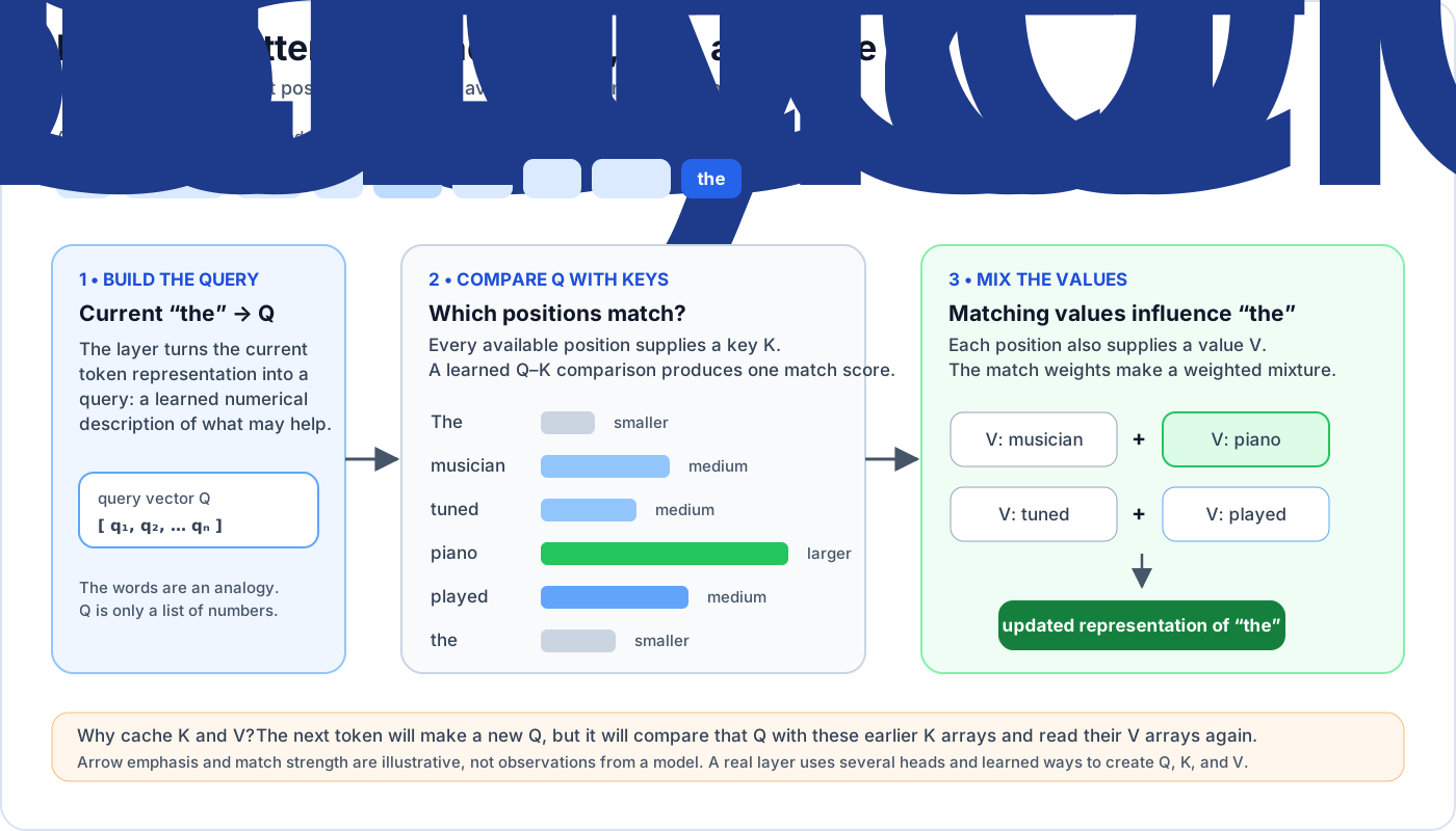
The names now explain the . A future creates a new query, compares it with the keys from earlier positions, and mixes the earlier values. It therefore needs the old keys and values again. It does not need the old queries: each old query already did its job when that earlier position was processed. That is why serving software K and V, not Q. The Transformer paper formally defines this query-key comparison and weighted use of values.
Prefill builds the first cache
During , the moves through the one layer at a . Within a layer, hardware can many positions together while the 's left-to-right rule prevents a position from using later positions. For every , each layer computes a key and a value. Serving software keeps them because a later output will need them.
The result is not one general-purpose note. It is a separate pair of numerical arrays for every layer:
layer 1 cache:  K and V for prompt positions 1 ... N
layer 2 cache:  K and V for prompt positions 1 ... N
...
last layer:     K and V for prompt positions 1 ... N
The same visible therefore has different saved at different layers. Those describe how that layer can match and use the position; they are not stored words, , or a plain-language summary.
Decode reads the cache and extends it
After selects the first output , repeats the following :
- Feed only the newly selected into the ; the earlier do not need to pass through every layer again.
- In the first layer, calculate a new query, key, and value for that .
- Compare its new query with the first layer's saved earlier keys and the current 's new key, then use the resulting to mix the corresponding earlier and current values.
- Keep the new key and value in the first layer's , making that layer's one position longer.
- Pass the result through the rest of that layer, including its .
- Repeat the same work in every later layer, using that layer's own . The current 's representation changes as it moves upward, so each layer calculates its own new query, key, and value.
- Turn the last layer's result into probabilities, select one , and begin the next step.
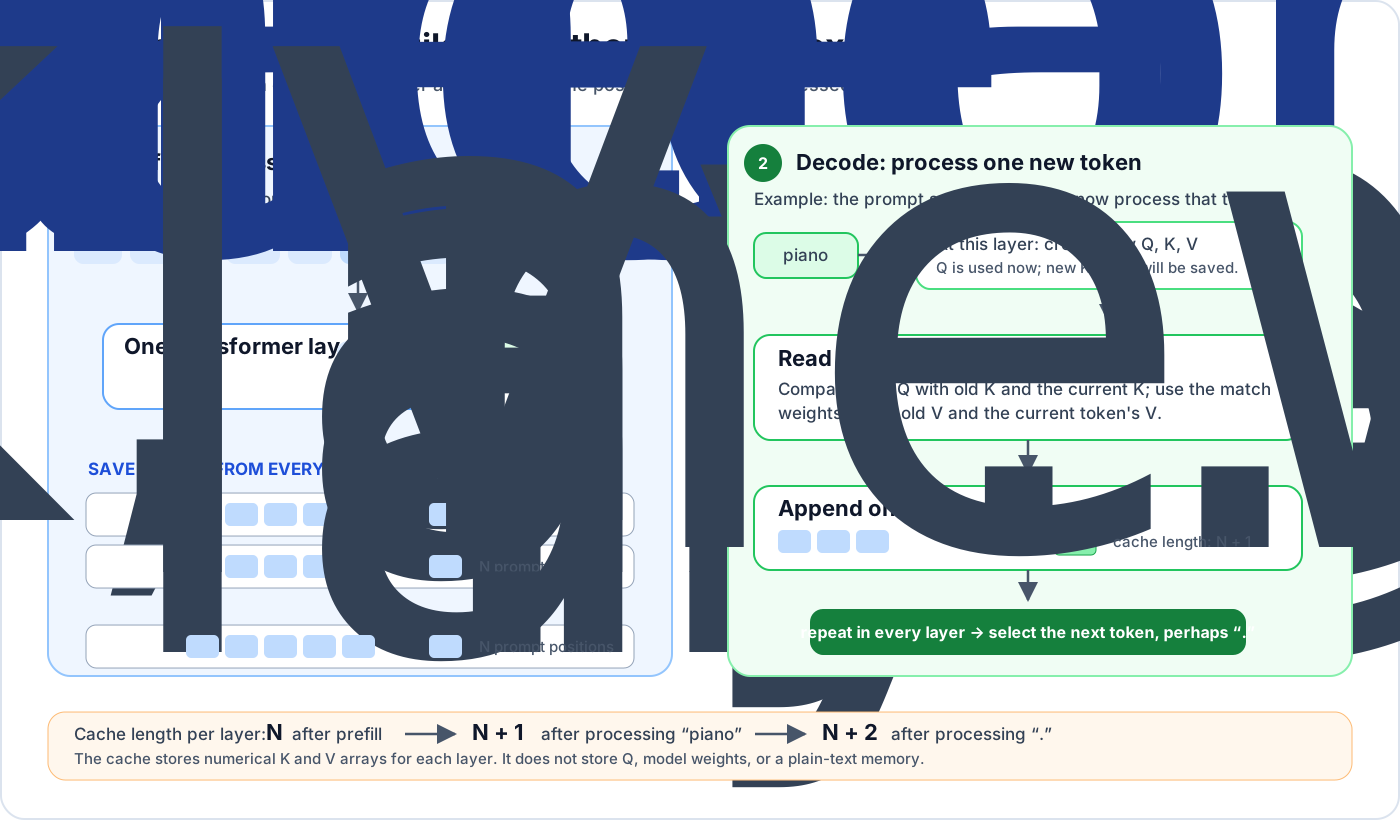
Return to the musician example. If the simplified contains N , creates N positions in every layer and the final position produces the scores from which piano is selected. On the next pass, the processes the newly selected piano, adds its key and value to every layer's , and may select a period. The now has N + 1 positions per layer. Processing the period adds one more position and produces another prediction. The sequence therefore grows N → N + 1 → N + 2, while the avoids rebuilding the first N sets of keys and values.
What the cache changes—and what it does not
| The does | The does not |
|---|---|
| keep each layer's earlier keys and values | keep a human-readable transcript or summary |
| avoid recalculating those earlier keys and values | replace the 's learned |
| grow as more positions are retained | make over the retained positions free |
| allow identical beginnings to be shared when serving software supports it | automatically remember material omitted from the 's current input |
The must still run its layers, create the newest query, key, and value, read the retained , and select the next . reuse changes duplicated work; it does not change the 's basic next- task. The also belongs to the current sequence. Each active sequence normally needs its own entries, although a serving system may share an identical beginning across requests. Hugging Face documents the per-layer cache and its growth, while the vLLM paper describes one production approach to managing and sharing .
A concrete memory calculation
size depends on the 's design, retained count, and used for each saved . Meta's Llama 3 report lists 80 layers and 8 key/value heads for its 70B . Its calculation splits an 8,192- representation across 64 , giving 8,192 ÷ 64, or 128, per head; each key/value head uses that same width. If each cached takes two , one retained requires:
80 layers
× 8 key/value heads
× 128 numbers per head
× 2 arrays (one key and one value)
× 2 bytes per number
= 327,680 bytes per retained token
≈ 0.328 MB per retained token
At 128,000 retained , those saved key and value occupy 41,943,040,000 , or about 41.9 GB in decimal units, for one sequence. For comparison, using the 's rounded 70-billion- label, stored at two each occupy about 140 GB. This comparison does not mean every deployment allocates exactly those amounts: software may reserve space in blocks, use a different , share an identical beginning, or retain fewer than the 's maximum .
The dimensions come from Table 3 of Meta's Llama 3 report; Meta's Llama 3.1 model card documents the 70B and its 128K- context. The durable lesson is the tradeoff: caching avoids repeated calculation, but a long retained sequence occupies substantial and still has to be read.
1.4 Serving Many Users Changes the Economics
Serving requests together can make an expensive cheaper per answer because one read can help several requests. The tradeoff is that each request consumes and may wait for a group to form.
First consider four users whose conversations are already in the phase. Without , the could handle them one after another:
without batching
read a block of weights → produce A's next token
read the same weights   → produce B's next token
read the same weights   → produce C's next token
read the same weights   → produce D's next token

with batching
read a block of weights once
        ├─ use it for A's next token
        ├─ use it for B's next token
        ├─ use it for C's next token
        └─ use it for D's next token
means processing several requests in one operation. The requests do not share answers or conversation histories. They share the opportunity to use the 's fetched before those are replaced by another block. This reuse performs more useful for each moved from , which can raise : total completed work per unit of .
A serving system usually cannot wait for four conversations to reach exactly the same point. Requests arrive at different , have different lengths, and some answers finish early. Modern serving software can therefore remove finished requests and add new ready requests between generation steps. The implementation details vary, but the purpose is the same: keep useful work on the without making an early request wait too long for a perfectly matched group.
has three limits:
- Waiting: Holding a request while a forms can increase its .
- : Every active sequence needs temporary state, including its own KV- entries unless an identical beginning can be shared. More simultaneous requests can exhaust before is full.
- Uneven work: A long or unfinished answer can outlast shorter requests. Serving software must replace finished work or leave part of the idle.
The result is a real tradeoff. A larger can lower cost per and raise total per second while increasing the delay one user sees. A useful serving report therefore gives both and user-facing under a stated request load. The vLLM paper documents one serving system that manages KV- in blocks and batches changing groups of requests.
1.5 From Chip Rental to Cost per Token
The useful economic question is not “How much does the chip cost per hour?” It is “How many acceptable outputs does that paid hour produce?” A cheap but mostly idle machine can cost more per answer than a more expensive machine kept productively busy.
There are three different prices that people often mix together:
| Price | What it includes |
|---|---|
| rental per hour | access to a stated amount of hardware for an hour |
| Provider cost per | rental or ownership plus the other resources needed to operate the service |
| price per | the price charged after overhead, service features, and margin |
The following calculation covers only the first row.
The basic conversion is:
raw accelerator-rental cost per million output tokens
    = total accelerator price per hour
      divided by tokens produced in one hour
      multiplied by 1,000,000
Suppose one rents for $2.20 an hour and the service produces 2,500 output each second across all users it serves at once. It produces 2,500 × 3,600, or 9 million output per hour. Dividing $2.20 by nine gives about $0.24 per million output . The result answers a narrow, hypothetical question: rental contributes about 24 cents per million output under those assumptions.
It is not the price. The provider must also pay for input processing, idle periods, networking, power, staff, failed requests, and profit. A low-delay chat service may use small batches and cost more. An overnight job may use batches and cost less. Long contexts may run out of before becomes the limit.
Any serving —a controlled performance test—should report three results: the delay before the first , the delay between later , and total per second across all users. It should also name the , hardware, input and output lengths, and of simultaneous requests. When only a few requests share a that uses all its groups, serving often streams much of the for each step. and KV- then strongly affect how many sequences can share an .
Part 2 — Training: How a Model Gets Its Numbers
changes a 's learned so its predictions improve. It repeats three steps: make a prediction, measure the error, and adjust the learned . Repeating this across enormous amounts of text requires substantial and extra for the information needed to make each adjustment. The learned state saved at a point in is called a . Initial commonly starts with randomly chosen values; continued or fine-tuning starts with values learned earlier.
2.1 A Trained Model Combines a Design With Learned Numbers
Code and configuration describe the 's design. learns its : numerical values saved in a . Many are entries in called ; others make different learned adjustments.
One participates in a calculation; it should not be read as one stored fact. Consider a made-up dot-product example:
inputs:   [2,  5, 1]
weights:  [3, -1, 4]

score = (2 × 3) + (5 × -1) + (1 × 4) = 5
The example multiplies matching values and adds the results. Many learned are arranged as rectangular arrays called . Multiplying a by a or another and summing products is called .
A applies learned calculations through a sequence of stages called . Most current use a design called a . A repeats blocks that include , the mechanism introduced in Part 1 for letting each use earlier text.
count is the publisher's count of individual learned . Suppose a 70-billion- stores every in two . The occupy about 140 GB. For comparison, the cited NVIDIA H100 configuration has 80 GB of , so that allocation cannot fit on one H100 without compression, , or moving some elsewhere. NVIDIA H100 specifications, accessed July 2026.
loads and uses learned . or fine-tuning changes them.
2.2 Training Is Repeated Prediction and Correction
A step does not simply tell the that an answer was wrong. It must calculate how each learned contributed to the error and then make a small coordinated adjustment. The is repeated prediction and correction:
For a made-up example, imagine that the text contains “The cat sat on the mat.” The sees “The cat sat on the” and assigns probabilities to possible next . If it gives “roof” 40 percent and “mat” 2 percent, it assigns little probability to the observed next , “mat.” A scoring rule turns that error into a . For the next- score used here, lower is better. It is called the .
The computation from input to prediction and loss is the . retains some intermediate values and may later recompute others because the next stage needs them.
The system then works backward through the connected calculations. For each , it estimates whether a small increase or decrease would make the loss better or worse, and by how much. That direction-and-size signal is called a . It is not the update itself. Calculating these signals backward through the is , usually shortened to the .
Finally, an uses the and an update rule to change . A widely used called keeps a moving average of each 's and another of its squared , then uses both when calculating the update. The original Adam paper defines these first- and second-moment estimates.
A is a group of examples processed together. A system can combine results from several smaller groups before one update. The rule rewards that make the observed answers more likely across examples. This differs from storing sentences as explicit database records, although a can still memorize and reproduce some examples.
2.3 One Formula Gives the Rough Arithmetic Bill
For a conventional that uses all its learned for every , work grows roughly with both size and the of . Double either one, and the estimated work roughly doubles. A useful estimate is:
training operations ≈ 6 × parameter count × training-token count
The source formula counts the main blocks separately from the learned tables that turn identifiers into starting representations and final scores. Those tables are usually a small share of a 's , so using the publisher's total count slightly changes the estimate. The shortcut also omits smaller and design-dependent calculations. Use it only for rough planning. Appendix F of DeepMind's compute-optimal training study gives the full accounting.
Why does the estimate contain the six? In the simplified accounting, the uses roughly two operations per for each : multiply a value by a , then add the result to a running total. The must calculate how the loss changes with both the layer's inputs and its , adding roughly twice the work. That gives about two operations for the plus four for the , or six in total. Real include operations that this shortcut does not count exactly, so six is an estimating rule, not a physical constant.
What does the rule predict for a run? For an illustrative 70-billion- trained on 15 trillion :
6 × 70 billion × 15 trillion
    = about 6.3 septillion operations (6.3 × 10²⁴)
One septillion is one followed by 24 zeros. To turn that intimidating count into elapsed , divide the work by the combined achieved rate of the :
time = total operations
       ÷ (number of accelerators × peak rate each × achieved share of peak)
Suppose 4,096 can each perform one quadrillion applicable operations per second using , a compact two- , and the complete run averages 40 percent of that theoretical rate. The division gives about 3.85 million seconds, or 44.5 days. At a hypothetical rental price of $2 per -hour, rent alone would be about $8.75 million.
Every figure after “suppose” is an illustrative assumption, not a report of a real run or market price. The example's purpose is to connect size and to and money: even thousands of fast chips can remain busy for weeks. Failures, storage, networking, preparation, and staff add work or cost. The one-quadrillion rate is rounded from NVIDIA's published H100 rate when every value is processed. A larger headline rate in the same table assumes a supported pattern in which the hardware can skip selected zero values. NVIDIA H100 specifications and footnote, accessed July 2026.
2.4 Training Needs Much More Memory Than the Finished Model
The main point comes first: can need far more than serving because it keeps the plus the information needed to update it. In one documented NVIDIA NeMo recipe, most calculations use , shortened to , a two- format that retains less detail. Updates keep a more detailed four- copy in , shortened to . Using more than one format this way is called . The in this example, , also keeps two running estimates for every . NVIDIA's NeMo 25.02 guide specifies two-byte parameters and gradients alongside four-byte master parameters and optimizer state, and the Adam paper defines its two per-parameter running estimates.
This illustrative setup keeps five items for every learned . The table explains why each one exists before adding their sizes:
| Item kept for one | Why it exists | in this example |
|---|---|---|
| working | used for most and backward | 2 |
| measures how the loss changes as the changes | 2 | |
| more precise master | receives the 's update | 4 |
| 's recent- average | helps smooth the update direction | 4 |
| 's recent-squared- average | helps scale the size of the update | 4 |
| Total | persistent state in this recipe | 16 |
The was introduced in Section 2.2, and the last two rows are 's running estimates. The important idea is that this recipe uses smaller values for much of the while retaining more detail for updates. Together, its five items use 16 per . Seventy billion therefore require 1.12 trillion , or 1.12 TB, before temporary results and software overhead. This is one worked recipe, not a law: other systems use different formats, , or ways of dividing and relocating .
An H100 with 80 GB of would require at least fourteen-way perfect division just to hold that 1.12 TB. A real run needs more devices because temporary values, communication buffers, uneven splits, and software must also fit. NVIDIA H100 specifications, accessed July 2026.
Splitting arrays so that each processor stores only a share is called . It saves on each processor, but the processors must exchange when a calculation needs the complete array.
also creates intermediate arrays of as the input passes through the network. These values are called . The needs selected , or enough information to recompute them. Their depends on the design, and length of examples, layer width, storage, how work is divided, and which values are saved.
The system can save a selected subset of intermediate values and recompute omitted operations during the . This , also called , trades extra for lower . The cost and saving depend on which operations are repeated; there is no universal percentage.
and therefore have different bills. may keep one compact copy of each plus the per-conversation from Part 1. The particular 16- setup above keeps eight as many persistent per as two- , plus . Other setups have different ratios. A chip that serves a well is not automatically the best chip for it.
2.5 Thousands of Processors Become One Fragile Machine
Adding processors shortens a run only when the extra parallel work outweighs communication, synchronization, imbalance, -loading, and failure overhead. At scale, network and reliability can materially limit completed work.
Start with a four- example. Each has an identical copy of the but reads a different quarter of a . All four perform the and backward passes at the same . They now have four different arrays because they saw different examples. Before any copy updates its , the add or average those arrays and give the combined result back to every participant. Only then can all four apply the same update and remain identical. This arrangement is .
The extra processors reduce the calculation each one performs on examples, but they add a communication step and a wait for the slowest participant. Other ways of dividing the create other exchanges:
There are several intuitive ways to divide a run:
| How the work is divided | What must be exchanged | Technical name |
|---|---|---|
| processors handle different examples; ordinary gives each a copy | combined before an update | |
| different processors hold different groups of layers | move ; signals showing how the loss changes move backward | |
| processors partition operations inside a layer | partial arrays combined through frequent communication | |
| processors hold different pieces of , , or state | pieces requested, combined, or moved when a calculation needs them | state |
runs combine these approaches. -parallel communication commonly occurs once per update or group of accumulated batches, while -parallel communication can occur several inside every block. The latter is usually more sensitive to link delay, but message size, the ability to calculate while moves, the connection layout, and the of processors all matter. Part 9 explains the resulting network hierarchy.
The table is a map, not a test. Processors can divide the examples, groups of layers, operations inside a layer, or stored and state.
Thousands of processors also make individually rare failures routine. In one 54-day Llama 3 snapshot, Meta recorded 466 interruptions: 47 planned and 419 unexpected. Unexpected interruptions therefore averaged one every 3.1 hours. The run used of up to 16,384 H100 . Meta's Llama 3 report, Section 3.3.4.
To recover, the system periodically saves enough durable state—such as , , schedule, and progress information—to resume from a saved point. This recovery differs from : one supports failure recovery, while the other reduces during a calculation. More frequent recovery can reduce repeated work after a failure but add storage, input/output, and synchronization overhead. The cited Meta report calls the share of wall-clock spent on useful “effective ” and reports more than 90 percent.
2.6 Training Continues After the Big Text Run
A trained only to continue broad text has learned a powerful next- task, but it has not automatically learned the behavior people expect from an assistant. If a contains a question and several possible continuations, the 's basic objective rewards likely continuations, not necessarily the most helpful, honest, or safe response.
Post- changes that behavior after the general run. A simplified looks like this:
- Show examples of desired behavior. Trainers prepare and suitable responses. Updating the on those pairs is .
- Compare possible responses. People, automated checks, or another may rank or score candidate answers. This creates preference or reward information.
- Train toward preferred behavior. A method uses that information to update the . from human feedback and are two different approaches; a real may use either, both, or neither.
- Evaluate and repeat. Developers test capabilities and unwanted behavior, revise or objectives, and produce another .
The InstructGPT paper documents one pipeline using supervised fine-tuning followed by reinforcement learning from human feedback, while the direct-preference-optimization paper introduces a different way to learn directly from preferred and rejected responses. These papers are examples, not a universal recipe.
For tasks with checkable outcomes, a system can generate candidate solutions and evaluate them with tests. is a broader family of methods that improves behavior to increase an expected reward; not every generate-and-filter is . Sampling candidates can make a substantial part of later .
A released contains fixed learned state that an service loads, often after conversion, , or . Ordinary does not update those . A provider may separately retain interactions and later use selected in another run, subject to its policy.
The distinction closes the loop:
training  = use data and an objective to update learned parameters
inference = use fixed parameters to compute outputs
is a concentrated project with a , , communication, and reliability bill. is the repeated cost paid whenever the file is used. Together they explain why hardware needs fast , spacious , quick links, dependable operation, and abundant power.
Part 3 — From a Prompt to Finished Work
In this course, an means software that repeatedly calls a and can use external . The proposes what to say or do next. A coordinating program, called the here, keeps task state, runs approved , returns their results to the , and decides when to stop. The itself does not click a browser or run a command; it produces text or a request that ordinary software may execute. A short answer may take one call, while research or coding can require many calls with searches, file reads, edits, and tests between them. “” has no single universal industry definition; this is the course's working meaning. OpenAI documents the model–tool–result flow here, and Anthropic distinguishes fixed workflows from agents here.
3.1 The Whole Agent in One Loop
The loop has five parts.
- The runtime gathers the material the needs: the user's request, relevant conversation history, instructions, available , and recent results. This bundle is the .
- The reads that context and produces either an answer or a proposed . A is a request such as “search for this phrase,” “read this file,” or “run these tests.”
- A well-designed runtime checks that the requested exists, validates its arguments, and enforces the user's permissions. A consequential action, such as sending an email or spending money, may also require explicit approval.
- If the call is allowed, the runs outside the . The search engine searches, the browser clicks, or the test runner runs. The returns an observation: a page, a screenshot, command output, a file, or an error.
- The runtime adds that observation to the task state and calls the again. The loop ends when the gives a final answer, the user must make a decision, or a safety or resource limit stops the task.
The loop is easier to see in a research task. Suppose the user asks for a comparison with sources. The first call may propose two searches. The runtime runs them and returns the results. The next call may notice that one source is a marketing page and request a more authoritative document. A later call may use a calculator. Only after the evidence is adequate does the write the answer.
3.2 What Happens During One Model Call
An task can contain many calls, and every call is a fresh request. The runtime must assemble the material needed for that call; the does not silently remember the result of an earlier call that the runtime leaves out.
Follow a simple research task. The user asks, “Compare two and cite the official specifications.”
- First call: The runtime supplies the request, instructions, and descriptions of available search . During , the processes those . During , it produces a request to search for the first specification.
- work: The runtime checks the request and runs the search outside the . The result might contain several links and snippets.
- Second call: The runtime sends the original goal plus the useful search result back to the . This call has its own and . The may request the official page rather than relying on a snippet.
- More and calls: The loop repeats for the second , calculations, and source checks.
- Final call: The runtime provides the evidence needed for the answer. The generates the cited comparison one at a .
call 1 context: goal + instructions + tool descriptions
call 2 context: goal + needed history + search result
call 3 context: goal + needed history + official specification
final context: goal + selected evidence + conclusions to check
The later contexts do not have to contain a verbatim copy of everything that happened. The runtime can retain exact evidence, summarize old discussion, reopen a source, or discard an irrelevant result. Each choice has a cost: dropping information can remove a needed fact, while carrying everything makes later longer.
The from Part 1 helps while a particular sequence is being processed and can sometimes let serving software reuse an identical beginning. It is not durable . The runtime still has to decide what information belongs in a later call.
Long tasks can therefore cost more in two ways: they make more calls, and later calls may more input . A rough task bill is the sum of every call's input and output cost plus paid and other services. Retries add to the bill even when they produce no useful final result.
End-to-end also includes work outside the . Tests, searches, websites, approval waits, and other services may take longer than . This is why the meaningful performance measure for an is usually the , cost, and success rate of a completed and checked task—not per second in one call.
3.3 Four Tasks, One Loop
| Kind of task | Typical shape | What usually slows it down | A useful success measure |
|---|---|---|---|
| Plain chat | One call, no | Reading the and generating the reply | to a correct answer |
| Research | Several calls with search and source reading | Finding trustworthy evidence and carrying it into context | Accurate answer with working citations |
| Coding | Repeated search, read, edit, and test cycles | Choosing the right files, test , and recovery from mistakes | A verified fix, not lines of code produced |
| Browser work | Repeated page-state or screenshot, decision, and action cycles | Page loads, changing interfaces, and permission checks | Correct completion without an unsafe action |
The economic lesson is simple: a low price does not guarantee a low task price. Suppose one takes 20 failed steps while another completes the same task in four; the lower price may still produce the higher total task cost. The are illustrative, not results. For work, track the cost, elapsed , and success rate of the whole task.
3.4 Further Reading
- OpenAI's function-calling guide shows the same -call, , result, and -call loop for software developers.
- Anthropic's guide to effective agents explains the difference between fixed workflows and systems in which the chooses its next action.
. An is not a new kind of . It is a repeated cycle in which the proposes, ordinary software checks and acts, and the result returns to the .
Part 4 — Why GPUs Suit Many Neural-Network Calculations
repeat the same calculations across arrays of . A graphics processing unit, or , is built to do many similar calculations at once; a central processing unit, or , is built to handle a wider variety of tasks and step-by-step decisions quickly. Neither is universally better: systems usually use for parallel and for operating systems, request handling, and serial control.
became a major -compute platform because their hardware and software fit many -network calculations. Other purpose-built processors use different designs for related work.
4.1 Two Ways to Be Fast
Imagine a supermarket deciding how to shorten its lines. It could hire one exceptional cashier who handles a difficult quickly, or it could open 100 ordinary checkout lanes for 100 with similar baskets. The first approach reduces the waiting for one complicated job. The second increases the of jobs finished each minute.
Computer designers call those goals and . is the elapsed for a specified job. is completed work per unit of . Both require a clear measurement boundary and unit.
High-performance cores devote substantial hardware to following irregular program logic and finding other instructions to run when one instruction must wait. Those features can reduce delay for work with many decisions and dependencies. also contain several cores and can perform parallel work, so “ favors ” describes a tendency, not a definition.
A organizes many small units into groups that normally receive the same instruction for different . Control hardware, nearby , and specialized units support that work. Performance depends on supplying enough similar work and avoiding too many different decision paths or waits for .
4.2 Graphics Supplied the First Big Parallel Job
did not begin as processors. They grew around a graphics problem: a screen contains many picture elements, or pixels, and many of those pixels need the same kind of calculation on different .
Consider drawing a lit red ball. Software first describes the ball's shape, position, and surface. The graphics processor then has to determine which screen locations the ball covers and what color each visible location should be. For thousands or millions of locations, it can apply related calculations to different coordinates, colors, and lighting inputs. Not every graphics step is independent, but the workload supplies far more similar operations than one general-purpose core could efficiently perform in sequence.
The useful progression is:
many screen locations
        → apply related calculations to different data
        → run many small workers in parallel
        → finish the image at an interactive rate
presented a different job with a similar hardware opportunity. Instead of calculating colors for many screen locations, they repeatedly multiply and add across arrays. The means something different, but the processor can again apply related instructions to many pieces of it at once.
turned out to contain many suitable operations. In 2012, an image-recognition network called AlexNet was trained on two and won a major image-classification contest by a margin. The original AlexNet paper reports the hardware and results. Image and language differ, but both contain array operations that can exploit parallel hardware.
4.3 Why Models Create So Much Repeated Arithmetic
Part 2 described a as learned organized into layers. Many of those sit in rectangular tables of called . A combines rows from one table with columns from another to make a new table.
Start with one row and one column:
row from the input:       [2,  5, 1]
column of learned weights: [3, -1, 4]

(3 × 2) + (-1 × 5) + (4 × 1) = 5
That multiply-and-add chain produces one in the output table. The next input row can be combined with the same column to produce another output . The same input row can also be combined with another column. A layer repeats this pattern across many rows and columns, creating a supply of related calculations.
                  weight columns
                 C1    C2    C3
input row R1  →  O11   O12   O13
input row R2  →  O21   O22   O23
input row R3  →  O31   O32   O33

O23 is built from input row R2 and weight column C3.
Many output positions can be worked on at the same because they use different row-and-column pairs. If a sum is long, workers can also calculate pieces of that sum and combine their partial results. This is the parallel structure that exploit.
Efficient software does not fetch every separately for every output. It loads small blocks of input values and into faster on-chip storage, uses each block for several output , then moves to the next block. Part 5 follows one of these blocks, called a , through the .
and in a use several , but a also normalizes values, applies other functions, coordinates , and moves . “ contain much ” is accurate; “a is only ” is not. The original Transformer paper specifies the learned projections used in and .
4.4 Moving Numbers Often Costs More Than Using Them
is only half the job. Before a calculator can multiply two , the must reach it. Bringing a value from can take more and energy than performing the multiplication that uses it. The exact difference depends on the chip and on how far the value travels, so there is no honest universal ratio. The durable conclusion is simpler: reusing a nearby value is cheaper than fetching it again from farther away.
Think of a kitchen. Chopping an onion is quick if the onion is already on the counter. If the cook must walk to a warehouse for every slice, adding more knives will not make dinner arrive sooner. A has many “knives.” Its central design problem is keeping ingredients close enough to use them.
shows how reuse helps. Suppose a small block of input contributes to eight different output blocks. A poor program could fetch that input block from eight . A better program fetches it once into small nearby and reuses it eight . The is unchanged, but seven long trips disappear. This is why layout and software can change speed even when the chip's peak stays the same.
That is why the next parts focus so heavily on and packaging. Several kinds of small sit on the chip, while high- beside it supplies much larger capacity. Software can keep temporary values in the smaller memories and reduce trips to the larger one.
Relative to a specified program and machine, work limited by traffic is ; work limited by is . can be , while generating text for only a few requests often becomes . These are common cases, not permanent labels for a .
4.5 Why CPUs Did Not Simply Keep Getting Faster
For decades, making smaller let designers fit more of these microscopic electronic switches on a chip while also raising clock speeds. Voltage could fall along with size, helping keep heat under control.
By about 2005, lowering voltage had become much harder and clock-speed growth slowed because of power and heat limits. IBM's history of Robert Dennard describes this transition. is a separate observation about growth in the of components that could be integrated economically; it is not a physical law. Intel summarizes Moore's observation and its later revision.
Power limits encouraged designers to spend additional on multiple cores and units specialized for particular calculations. already existed; the power limit accelerated parallel and specialized computing rather than causing to be invented.
Further reading:
- 3Blue1Brown's neural-network lessons show visually how repeated multiply-and-add operations become a network.
- Mark Horowitz's energy-cost presentation compares the energy used by and by movement in one documented chip technology. Its figures are historical examples, not constants for current hardware.
What to remember: A is not a universally faster . Its -oriented execution and system make it effective when a workload exposes enough similar parallel operations. Many -network operations do; other portions can remain limited by serial work, , or communication. The next challenge is feeding the parallel hardware with .
Part 5 — What Happens Inside an AI Accelerator
An is useful only when its units receive and ready work. The practical limit may be , traffic, or coordination among many pieces of work. This Part explains those three possibilities before introducing any vendor-specific names.
Think of a factory. units are workers. Tiny on-chip memories are workbenches. The 's device is the stockroom. A is control hardware that chooses which ready group of work runs next. This analogy describes the roles, not a literal map of every .
5.1 A GPU Repeats the Same Small Factory Many Times
designers repeat processing blocks across the chip's piece of silicon, called a . Repetition matters because one block can handle one portion of an array while other blocks handle other portions at the same .
Follow one piece of a :
- Software divides the into small blocks of work.
- Control hardware assigns a ready block of work to a processing block on the .
- Workers in that processing block load needed into and small shared working .
- paths and engines multiply and add those .
- The block writes completed results to the larger device or passes them to another calculation.
Each processing block contains paths, scheduling hardware, for immediate values, and a small amount of on-chip working . Different blocks can be at different points in this sequence while sharing a larger system.
A keeps copies of from a slower . It helps when a later access finds the needed value there, so software often arranges work to reuse nearby . Exact block and names vary by vendor; the stable idea is repeated parallel processing supported by a hierarchy of local storage. NVIDIA's programming guide and AMD's hardware glossary document two concrete designs.
5.2 Many Workers Can Share One Instruction
One hardware path can perform an operation on one set of values. reduce control overhead by giving a common instruction to a group of small workers, which apply it to different . Group names and sizes vary by vendor.
Imagine a group of bakers receiving the instruction “add two cups of flour,” each for a different bowl. One instruction coordinates many useful actions. This is efficient when every bowl needs the same step. It becomes inefficient when half the bakers need to whisk while the other half need to wait; the group may have to perform both paths in turn.
The rule underneath matters more than the labels: are most efficient when workers in a group need the same instructions. If they take different decision paths, the hardware must handle those paths separately while some workers sit idle. Modern NVIDIA hardware does not require every worker to advance in literal “lockstep,” so that familiar shorthand is misleading. NVIDIA GPU programming guide.
5.3 The Chip Switches Jobs While Data Is in Transit
Device can take much longer to respond than an operation. A cannot remove that delay, so it keeps multiple thread groups ready. When one group waits for , the scheduler can issue work from another ready group.
Think of a restaurant server with several tables. After placing one table's order with the kitchen, the server does not stand still until the food appears. They take an order from another table, deliver a drink to a third, and return when the first meal is ready. Enough independent tables keep the server productive despite each kitchen delay.
Engineers call this : working on something else during a delay. A simplified timeline looks like this:
group A: request data ───────── wait ───────── calculate
group B:          calculate → request data ───── wait
group C:                     calculate → request data

processor: useful A/B/C work fills some of the waiting periods
The response did not become faster. The processor merely found independent work that was ready. succeeds only when the program supplies enough such work and each group leaves enough and on-chip for other groups to remain ready. If one group consumes nearly all nearby storage, too few alternatives may fit. If every group waits on the same missing result, there is nothing to switch to. NVIDIA's GPU programming guide documents hardware scheduling and the resource limits on active thread groups.
5.4 Special Matrix Engines Do the Main AI Calculation
Modern contain specialized circuits for the repeated work from Section 4.3. NVIDIA calls its versions ; other vendors use other names. A is not a separate processor that runs a whole . It is an unit inside the that performs a supported operation on small blocks of .
The handles a in pieces:
- Divide the input and into small rectangular blocks called .
- Load matching from device into faster on-chip storage.
- Give those to a engine, which performs many multiply-and-add steps.
- Add the partial result to the output . A output may need contributions from several pairs of input .
- Reuse any that contributes to another output, then store the completed output .
large input matrix     large weight matrix
┌───┬───┬───┐          ┌───┬───┐
│ A │ B │ C │          │ D │ E │
└───┴───┴───┘          └───┴───┘
       ↓ choose matching tiles
     matrix engine performs a small matrix operation
       ↓ repeat and add partial results
          one output tile
The exact shapes, accepted , and instructions depend on the product. The stable idea is that dedicated wiring can perform a common block of more efficiently than issuing every multiply and addition as an unrelated instruction.
Specification sheets usually report the highest theoretical rate for a stated —the rule used to encode in —and may assume a supported pattern of zeros. Code must use a supported operation and keep the unit supplied with to approach that rate. The therefore does not describe arbitrary code or guarantee application speed. NVIDIA's H100 table illustrates how the stated rate changes with format and sparsity; its programming guide describes -core operations.
5.5 Local Memory Has Several Levels
Within one , storage levels trade capacity and chip area against access and :
closest to arithmetic

registers             immediate values for individual threads
on-chip working memory  small reusable tiles for one processing block
caches                copies of data from larger memory
device memory         model weights and other large arrays

farther from arithmetic
are tiny storage locations used directly by instructions. The next levels use a fast on-chip technology explained in Part 6. device uses other technologies introduced there. Exact sizes, names, and access costs depend on the .

on another , the main computer's , and storage are separate pools reached through additional links. They are not extra rungs with guaranteed increasing capacity, and their order can change by product and by whether the reader compares delay or transfer rate. Fast software loads useful into nearby storage, reuses it, and avoids unnecessary transfers.
5.6 Every Operation Faces One of Two Ceilings
To predict whether a piece of code will run well, ask two questions:
- How much does it perform?
- How much must it move to perform that ?
If an operation uses each fetched value many , the units may become the limit. Adding faster will not help much because the calculators are already full. The operation is .
If an operation does little work with each fetched value, arrives too slowly to fill the calculators. Adding more units will not help much because the existing ones are waiting. The operation is .
Engineers measure work per transferred across a named boundary as . The simplified gives this upper bound:
attainable arithmetic rate is no greater than the smaller of:

1. peak arithmetic throughput
2. memory bandwidth × arithmetic operations per byte
operations in and processing often reuse values enough to become . When only a few requests share a that uses all of its groups, generation can do relatively little work per of read and become . design, context length, of simultaneous requests, software, and hardware can change either result.
Use a small illustrative machine to see the rule. Suppose it can perform at most 1,000 operations per second and its supplies 100 per second.
- An operation that does two steps per can be supplied with at most
100 × 2 = 200operations per second. sets the lower ceiling, so the operation is . - An operation that does 20 steps per has a ceiling of
100 × 20 = 2,000operations per second. The machine can perform only 1,000, so sets the lower ceiling and the operation is .
The same operation can move from one side to the other when software increases reuse, the reduces , or the machine changes. The label belongs to a particular workload and implementation on a particular system.
Real programs can fall below both ceilings because of coordination, scheduling, or other overhead. The tells you which resource sets the best possible limit; it does not promise that software reaches it.
5.7 Better Software Can Remove Entire Memory Trips
A is a small program the runs across many parallel workers. A simple implementation may run one , save an intermediate result to device , then run another that immediately reads it back.
combines compatible steps so the intermediate result can be eliminated or remain in , on-chip working , or :
separate steps:
device memory → step 1 → device memory → step 2 → device memory

fused steps:
device memory → step 1 + step 2 → device memory
Fusion can reduce traffic and the work needed to start separate programs, but using too many on-chip resources can make it slower. FlashAttention is a real example: it reorganizes so less moves between and small on-chip while producing effectively the same result. Reordering calculations can still create tiny numerical differences.
This is why software support is part of practical hardware performance. Libraries and compilers choose operations, layouts, reuse, fusion, and scheduling. Peak specifications give a ceiling under stated conditions; an application reaches only what its full implementation sustains.
Further reading:
- The original Roofline report defines the two-ceiling performance .
- The FlashAttention paper is a primary-source case study in reducing traffic.
What to remember: A groups into repeated processing blocks, keeps several thread groups ready to cover delays, and uses engines for supported operations. Whether compute, local traffic, or coordination is the tightest limit depends on the workload and implementation.
Part 6 — Memory: What Fits and How Fast It Moves
has two separate jobs. It must be enough to hold the and its temporary working , and it must deliver those quickly enough to keep the processor useful. The first property is . The second is .
Think of a water system. Capacity is the size of the tank; is the width of the pipe. A tank with a narrow pipe stores plenty but delivers slowly. A wide pipe attached to a small tank delivers quickly until the tank runs out. systems often need both a tank and a wide pipe.
6.1 Fast Memory Is Small; Large Memory Is Farther Away
No single kind of gives a processor unlimited capacity, immediate access, low power, and low cost. Designers therefore build a hierarchy: a little fast storage close to the and much more storage farther away.
, , and small working memories on a processor commonly use static random-access , or . An cell keeps its while power remains available without the periodic refresh used by . That makes it useful for fast on-chip access, but its circuit uses more and chip area for each stored . Filling a with enough for a would therefore require far more silicon area and cost than present designs can justify.
device memories use dynamic random-access , or . A cell stores charge that must be sensed and refreshed. Its denser design fits more in a given area, but access involves more delay than the small on-chip memories. In high-end , is manufactured on separate and connected to the processor through the . Samsung's memory overview explains storage and refresh and compares its density with .
The useful analogy is a desk and a nearby library. The desk is fast to reach but holds only today's working papers. The library holds far more, but every visit takes . Good programs bring a useful set of papers to the desk, work with them repeatedly, and return them only when necessary. Sections 5.4 and 5.7 described exactly this strategy with and fused calculations.
High- , introduced next, is arranged and connected through an unusually wide interface. It is not a different storage principle.
6.2 High-Bandwidth Memory Uses Many Short Wires in Parallel
High , or , raises transfer rate mainly by moving over a very wide set of short connections. Instead of asking a comparatively small of wires to run at ever-higher rates, the carries many pieces of in parallel.
One stack is assembled in stages:
- Several store the actual .
- The are stacked, and vertical paths connect the layers.
- A base or interface layer connects the stack to the .
- Dense wiring links the stack to the 's compute .
- A controller on the processor coordinates reads and writes across the wide interface.
The is close to the processor in the , but it is not part of the processor . still has to travel through cells, the stack, wiring, and the processor's system before units can use it.
Graphics Double Rate, or , devices are commonly mounted around a on a circuit board. uses narrower connections that transfer at a higher rate on each wire than . Neither name alone establishes which product is faster, larger, or cheaper; exact capacity and depend on the generation, of devices, interface width, and complete system.
That wiring is not always one full silicon layer. Current designs can use a silicon wiring layer, fine patterned wiring made from other materials, or small local silicon bridges. capacity therefore depends on - fabrication, stacking, routing, assembly, and test—not simply attaching a conventional module. SK hynix explains the stacked memory and vertical connections, while TSMC documents several package-wiring approaches.

6.3 Capacity Answers “Will the Model Fit?”
Suppose a contains 70 billion and stores each one in two . The payload is 70 billion × 2 = 140 billion bytes, or 140 GB in decimal units. Those alone exceed the 80 GB in the cited H100 configuration and fit within the 192 GB in an AMD MI300X. NVIDIA H100 specifications and the AMD MI300X data sheet provide those capacities. Complete also needs temporary workspaces and usually a , so 192 GB does not guarantee that every group of requests and context length fits.
The order of the check matters:
available device memory
    − model weights
    − KV cache for active sequences
    − temporary workspaces and software allocations
    = remaining safety margin
If that result is negative, the service cannot simply “run a little slower” on the same allocation. It must change what is stored or where it is stored. Section 1.3 calculated about 41.9 GB of for one 128,000- sequence on a specific 70-billion- . This is why a whose fit can still run out of as context length or size grows.
If all required does not fit, a system can split selected state across , move some state to slower , reduce numerical , shorten the context, or choose a smaller . These choices can add communication, delay, software work, or quality loss. Capacity can therefore change the architecture and cost of the system.
needs more than . It commonly stores , state such as 's running averages, and intermediate arrays called . Systems can divide some state among . , also called , saves only selected intermediate results and recreates others during the , trading extra calculation for lower use. PyTorch documents that trade.
The plain-language rule is: when is scarce, engineers either divide the , store it more compactly, or repeat some calculations instead of storing their results.
6.4 Bandwidth Answers “How Fast Can the Model Be Read?”
When only a few requests share a that uses most of its for every output , each generation step may stream most of the while doing relatively little work per . can then be the limit. Serving more requests together can share a read, and other designs can change how much moves.
If a step must read a 140 GB file once, an ideal 3,000 GB/s interface could supply at most about 21.4 complete -file reads per second: 3,000 ÷ 140. This uses decimal units and assumes peak , one full read per step, no competing traffic, and no communication or overhead. One low- stream will normally be slower. Aggregate per second can be higher when a shares each read, so this is not a universal -rate ceiling.
This example gives the a question and a baseline. “Three terabytes per second” sounds enormous in isolation. Compared with a 140-gigabyte that must be revisited after , it becomes a limit the reader can feel.
The widening gap between processor and -system speed is called the . and reuse reduce external- traffic, lower reduces moved, and wider interfaces such as raise . Which response helps depends on the workload. Wulf and McKee introduced the term.
6.5 Memory Supply Can Limit Accelerator Supply
An vendor cannot ship an product merely because a processor exists. The required must pass through its own chain:
make DRAM dies
    → test them
    → assemble and connect the stack
    → test the stack
    → qualify it for the customer's platform
    → assemble and test the complete accelerator package
An stack contains multiple , many vertical connections, and an interface layer that joins it to the . A failure in a , connection, stack assembly, or later can reduce the of usable finished parts. Testing at several stages can reduce the chance of assembling a component already known to have failed, but it cannot remove every integration risk.
production and —testing that a component meets a 's platform requirements—are specialized stages. Too little production, too many rejected stacks, or slow qualification can therefore reduce usable supply even when processor are available. Supply claims should always name the generation and date.
For a reader following the industry, the practical questions are straightforward: How much does each carry? How quickly can it move that ? How many tested stacks can suppliers produce? Those three questions connect the , the hardware, and the supply chain without requiring a catalog of version names.
Further reading:
- SK hynix's HBM explanation covers stacked , vertical connections, and the wide interface.
- The AMD MI300X data sheet is a concrete example of how capacity and appear in a product specification.
What to remember: Capacity determines whether and working fit. limits how quickly can supply . raises with stacked and a wide interface, adding demanding , assembly, test, and packaging stages.
Part 7 — Why AI Uses Smaller Numbers
Many and systems store or compute some arrays with fewer while retaining more detail where it is needed. Fewer can reduce storage and traffic and can increase on matching hardware. Smaller formats can erase fine differences between nearby values or fail to hold outside their range. Either problem can change quality, so the usable format depends on the , task, and operation.
The practical question is not “What is the smallest format?” It is “Which format meets the measured quality target for this workload?” A performance claim is incomplete without the format, quality result, and measurement conditions.
7.1 A Number Format Divides Bits Between Range and Detail
Computers store as patterns of , the zero-or-one values introduced in Part 0. More allow more possible patterns. Designers must decide what those patterns mean.
For values that can be extremely or small, computers commonly use a scheme similar to scientific notation. The decimal expression 3.14 × 10² separates significant digits from scale. A binary format likewise records a sign, a scale, and meaningful digits.
The two jobs are range and detail. Range determines how or small a magnitude the format can represent. Detail determines how closely it can distinguish nearby values at a given scale.
Imagine a tiny decimal format that keeps only three significant digits. It can store 3.14, but the value 3.14159 must be rounded. Near 3, it cannot distinguish every possible value between 3.14 and 3.15. A format with more significant digits can preserve more of that difference. Separately, a larger exponent field lets the format move the decimal—or, in a computer, binary—point across a wider range of magnitudes.
Giving more to the exponent therefore allows a wider range of sizes. Giving more to the significant digits preserves finer differences between nearby values. Reducing the total of makes storage and supported cheaper, but it increases rounding and the chance that a value is too or too small to represent.
The IEEE 754 standard, published by the Institute of and Electronics Engineers, defines a 32- format called binary32. It is commonly called and uses four . uses 16 , keeps a similarly wide range, and records less fine detail. names a family of one- formats with different balances between range and detail. Four- formats use half a per value only when packed tightly; scaling information and other metadata add storage. IEEE 754, Google's BF16 guide, and the FP8 formats paper define these distinctions.
7.2 Smaller Numbers Save Space, Movement, and Arithmetic
For 70 billion , the packed payload alone requires roughly the following in decimal gigabytes. Metadata, padding, , workspaces, and other runtime state are excluded:
two bytes per weight:       140 gigabytes
one byte per weight:         70 gigabytes
half a byte per weight:      35 gigabytes
Reducing the payload from two to one changes 140 GB to 70 GB, so the alone fit within an 80 GB device. The complete service may not fit once metadata, , workspaces, and other allocations are included. If traffic is the only limit, halving those gives an ideal bound near twice the -delivery rate; real speedup may be smaller. Supported low- units can also have higher stated .
maps values from a larger set into a smaller set of representable values. Picture taking many precise temperature readings and recording each one at the nearest whole degree. The record becomes simpler, but several slightly different readings now share one stored value. uses more sophisticated mappings and commonly stores scaling information for groups of values, but the central tradeoff is the same: fewer stored choices mean less and more approximation.
may apply to , temporary values, or the . It can reduce storage and traffic and accelerate supported calculations, but quality and speed depend on the method, , task, and hardware. PyTorch's quantization overview explains the mapping and scale used to represent a larger numeric range with fewer .
repeatedly updates and must represent and accumulated state, so recipes often retain more for selected values. often permits aggressive -only , but acceptable remains - and task-specific. “Supports 4- ” does not establish that an entire or workload used four at acceptable quality.
7.3 How to Read an Accelerator Specification Honestly
Start with the workload, then compare matching measurements. Five questions remove most of the confusion:
- What kind of entered the calculation, and what kind held the running total? Compare rates only when both formats and the operation are the same.
- Does the peak assume that zeros appear in the exact pattern the hardware can skip? This is called . Compare results under the same condition; arbitrary zeros do not automatically earn the advertised speedup.
- Is the total for one processor , one server, or a whole rack? A larger box naturally produces a larger headline.
- Does the workload need , , or most? Peak operations per second cannot answer the other two questions.
- What happened on a real at an acceptable quality and response ? A is more informative than a theoretical ceiling when its setup matches the intended use.
Report power or energy beside and because a power-constrained facility may care about work per watt or per rack. Report software and versions because application performance depends on the available , compilers, and libraries.
A useful comparison therefore holds operation, format, sparsity assumption, workload quality, and measurement conditions constant. It reports , and , link and , power, application , and response .
Further reading:
- The Institute of Electrical and Electronics Engineers' floating-point overview is the formal source for conventional formats.
- NVIDIA's low-precision primer explains how multiplication with smaller formats is combined with scaling and a more detailed running total.
What to remember: Fewer can reduce packed size and traffic and can raise on supported hardware. They can also reduce measured quality. Compare the same operation, format, sparsity assumption, workload, and quality target—not the largest on a slide.
Part 8 — How an Accelerator Is Manufactured
This Part focuses on high-end -center that use . A is one piece of processed silicon containing a circuit. A protects and connects one or more to the rest of the system; some also contain nearby stacks. is the separate assembly work that joins these pieces with dense wiring.
Finished supply therefore depends on processor , qualified , assembly, and test. A shortage, high rejection rate, or qualification problem at any required stage can limit finished even when the other parts are available. Intel defines die and package, while TSMC documents current HBM package structures.
8.1 Start With What the Workload Requires
An is easier to understand when you start with the problems it must solve. The is not an arbitrary collection of silicon pieces; each major part answers a workload need.
The compute contains the engines, general paths, control hardware, and on-chip introduced in Part 5. stacks supply much larger and . Dense wiring below and between those components carries many closely spaced signals that would be difficult to route across an ordinary server board. Other circuits bring in power and connect the to the rest of the server.
Seen from above, the result resembles a small city center. The main processor sits in the middle. stacks sit around it. A dense wiring layer underneath carries traffic between them, and a larger base connects the whole assembly to a server.
This city picture describes one common arrangement, not every . A need not contain , and different products place and connect their components differently.
8.2 From a Silicon Wafer to Individual Dies
Chip fabrication turns a blank silicon into many copies of an intricate circuit. It does not carve a complete with one tiny . Instead, the factory builds and connects structures layer by layer through a repeated sequence of coating, patterning, adding, and removing material.
A simplified journey is:
- Prepare the . Fabrication starts with a circular of highly purified silicon. For scale, Intel says the modern it uses are 12 inches, or 300 millimeters, across. Intel's manufacturing glossary supplies that example.
- Add a light-sensitive coating. This coating changes where light reaches it.
- Project one circuit pattern. uses light and a patterned mask to expose selected areas. Developing the coating leaves a temporary pattern on the .
- Change the exposed material. Other equipment can remove material, add a thin material, or change selected properties. The exact operation depends on the layer being built.
- Repeat for many layers. form first, and later conducting layers connect them into circuits. Each layer must line up with the earlier ones.
- Test and separate the . Probe tests identify that meet specified limits. The is cut, or diced, into individual . Acceptable continue to packaging and further tests.
Leading-edge processes use extreme-ultraviolet light for selected critical layers; other layers can use different systems. ASML explains the coat, expose, develop, and repeated layer process, including deposition, etching, and other steps omitted from this introduction.
The steps above omit hundreds of specialized operations and inspections. The mental is what matters: one carries many repeated circuits, each circuit is built through many aligned layers, and a finished still has to be tested and divided. Some designs can disable a faulty repeated block and still meet a supported lower configuration; that meet no supported specification are discarded.

Many companies design chips but hire a specialist manufacturer, called a , to make them. This is why one 's plans can affect several competing chip companies.
8.3 “3 Nanometer” Is a Generation Name, Not a Measurement
Foundries give manufacturing generations names such as 7 nanometer, 5 nanometer, or 3 nanometer. This named generation is a . Modern node names do not measure one physical feature, and labels from different foundries cannot be compared directly.
That means a chip sold as “3 nanometer” does not contain one important part that is simply three nanometers wide. Decades ago, node labels tracked particular device dimensions more closely. Modern and their wiring have several relevant dimensions, and manufacturers use node names to distinguish a generation of design and manufacturing technology.
For a specific design, compare how many circuits fit, how fast and energy-efficient it is, what share of pass testing, and what it costs. A newer may improve some combination of those properties, but the result depends on the circuit and design choices; development, masks, , and packaging can also cost more.
When two products use different nodes, replace “which nanometer is smaller?” with four questions:
- How does the complete chip perform on the same workload?
- How much power does it draw to produce that result?
- How and costly is the finished and ?
- How many usable parts can the manufacturer produce?
Smaller labels therefore do not guarantee a cheaper finished . A designer may use the available for more , control, , or links, subject to area, power, and cost limits. On-chip has also become harder to shrink. Treat the node as one manufacturing input, not a product performance score. Intel explains modern node naming.
8.4 Bigger Dies Are Powerful but Harder to Produce
Two limits make a expensive.
First, a scanner can print only a limited rectangle at a . This constrains the size of a conventional made in one exposure area. ASML system specifications.
Second, microscopic defects occur during manufacturing. Picture cutting brownies from a tray that contains a few burnt spots. If the brownies are small, each burnt spot ruins one small piece and many good pieces remain. If the brownies are huge, the same spot can ruin a much more valuable piece. have the same problem.
The circle creates a separate loss. Rectangular near a 's edge do not fit completely, so a larger rectangle also tends to produce fewer complete candidates from one . Defects then reduce that candidate count further. The exact result depends on dimensions, layout, defect distribution, and which faults the design can tolerate; the analogy explains the direction, not a yield formula.
is the share of manufactured that meet required tests. Designers may include redundant or disable-able blocks so a with a localized defect can still meet a supported configuration. Manufacturers then test and sort acceptable parts into product or performance grades; that sorting is . A lower bin may be fully functional but unable to meet a higher speed or power grade.
These effects are why a count does not translate directly into the same of premium parts and why related products may expose different of working units. Yield, defect tolerance, and are related but not interchangeable ideas. Intel's manufacturing glossary.
8.5 Chiplets Trade One Large Problem for Several Smaller Ones
When one becomes too hard to print or too wasteful, designers can split it into several smaller and connect them inside one . These pieces are called .
The brownie analogy shows one potential benefit: a localized defect affects a smaller piece. can be tested before assembly to reduce the chance of packaging a bad part. A can also combine made with different processes—for example, newer with mature circuits that move into and out of the . Total economics still depend on how many assemblies pass testing.
Imagine a design that needs four repeated regions. A one- version places all four on one rectangle. A version manufactures four smaller and joins acceptable ones in a . A defect that ruins one small does not automatically discard the other three before assembly, and the factory can test the pieces first. But the finished now needs working links among all four pieces, enough wiring to carry their , and a way to deliver power and remove heat across the assembly.
add -to- communication, routing, power, thermal, assembly, and test requirements. Crossing a boundary can cost more delay and energy than communication within one , although the exact cost depends on the interface and . Hardware, firmware, compilers, or application software must manage whichever parts of this layout they can see. move part of the problem from one into integration. UCIe documents one standardized die-to-die interface.
8.6 Advanced Packaging Joins the Processor to Memory
Fabrication produces separate compute and . turns those pieces into one usable by placing, connecting, protecting, powering, and testing them as an assembly.
Follow one read from . A cell in an supplies through the stack's vertical connections. Signals pass through the stack's interface and across dense wiring to the compute 's controller. The controller delivers the requested into the processor's hierarchy, where units can finally use it. Every physical connection on that path must work at the required rate.
An ordinary server board cannot directly route all of the closely spaced signals needed by a wide interface. Vendors therefore use denser wiring, such as a silicon , fine patterned wiring made from other materials, or small embedded silicon bridges. An is an intermediate routing structure between components; it carries signals but does not perform the 's .
The assembly sequence varies by product, but the dependency is universal: good compute and good stacks are not finished until the joins them and passes test. Packaging therefore has its own equipment, capacity, yield, and qualification limits. TSMC documents several current wiring approaches and their processor-to-HBM arrangements.
A finished therefore depends on processor- fabrication and test, - fabrication, stacking and test, assembly and test, and later board or server integration. A shortage, high rejection rate, or qualification delay at any required stage can limit usable systems.
Further reading:
- ASML's lithography overview explains how circuit patterns reach a .
- TSMC's CoWoS overview distinguishes silicon-, redistribution-layer-, and bridge-based structures.
What to remember: A usable depends on processor , , packaging, test, and system integration. Larger can reduce . can reduce one - risk but add integration work. The tightest required production stage can constrain finished supply.
Part 9 — Why Multiple Accelerators Need Fast Connections
and jobs are often divided across . Communication then becomes part of the calculation, and a processor can sit idle while it waits for another one.
Designers try to keep frequent, delay-sensitive communication inside a tightly coupled group and use the broader network across servers or groups. The first arrangement is called ; the second is . They describe system organization and communication scope, not simply two physical distances.
9.1 Scale-Up Makes Nearby Accelerators Behave Like One Larger Machine
Imagine four people assembling one puzzle. If they sit at the same table, they can pass pieces and point to matches with little delay. If each person sits in a different building, the same coordination becomes much slower even if every person works equally fast.
networks connect a tightly coupled group with links designed for high and low delay. NVIDIA calls its version NVLink and uses switch chips to extend it across supported systems. Other vendors use other designs. A group may be inside one server or extend across a rack; software must still divide and coordinate the work.
networks connect servers or groups through switches. is a standardized family of -center network technologies. is a switched network design built for high -transfer rates and short delays. A path often provides less to each and more delay than the local network, but exact rates, sharing, and connection layout depend on the deployed system. NVIDIA documents NVLink, and the InfiniBand Trade Association documents .
scale-up: a tightly coupled accelerator group

   [GPU] ===== [GPU]
     ||           ||
   [GPU] ===== [GPU]

scale-out: many servers and racks, network switches between them

   [server] --- [switch] --- [switch] --- [server]
Neither layer replaces the other. A —a group of connected computers managed for shared work—can use tightly coupled groups and then connect those groups over a broader network.
9.2 Compare Each Communication Path Directly
For a specified system, compare local , the fabric, and the network separately. Local commonly supplies the most per , but there is no universal ratio or ordering for every metric. Product, direction, , link count, and whether a figure is per port or an aggregate all matter.
The safe lesson is conditional: when the same value is already in local , using it usually avoids a link transfer. When is remote, ask how many cross which link, how often, and whether the quoted rate is theoretical or measured.
That is why “the fits across eight ” is not a performance result. If the devices exchange arrays after nearly every layer, communication can dominate running . If they work independently for longer periods and exchange small summaries, a slower path may be adequate.
Consider a simplified divided across two . A holds the left half of a and B holds the right half. Both receive the layer's input and calculate different parts of the output at the same . If the next calculation needs the complete combined result, the two devices must exchange or combine their partial arrays before either can continue.
same layer input
   ├─→ accelerator A uses weight shard A ─→ partial result A ─┐
   └─→ accelerator B uses weight shard B ─→ partial result B ─┤
                                                              ↓
                                                    exchange/combine
                                                              ↓
                                                      next calculation
The may take less because two processors share it, yet the layer now includes a communication step. If that exchange takes longer than the saved calculation , adding the second makes the layer slower. Real -parallel layouts split particular and use different collective operations, but the dependency is the same: the next step sometimes cannot begin until remote partial results arrive. The Megatron-LM paper gives a primary-source example of splitting -layer operations across .
Placement should follow measured communication: keep high-volume, delay-sensitive exchanges on paths that meet their needs, and spread more independent work across the broader network. The connection layout is part of the workload design, not a decorative server specification.
9.3 Group Communication Has Repeated Patterns
In -parallel , each worker processes a different group of examples and computes : arrays describing how the loss changes with the . Before the next update, the workers combine those arrays so their copies remain in agreement.
An combines every participant's array with a chosen operation and returns the combined array to every participant. Suppose four workers calculate one illustrative value:
worker A: 2       worker B: 4       worker C: 6       worker D: 8
                         all-reduce with addition
                                      ↓
every worker receives: 2 + 4 + 6 + 8 = 20
framework forms the average if needed: 20 ÷ 4 = 5
Real are arrays, not one . A communication library divides those arrays into blocks, moves blocks along available paths, and combines them. The operation is collective because every worker participates and every worker needs the result. Addition is common for , but the standard supports other reduction operations. The message-passing standard defines all-reduce.
An moves different rather than one combined result. Each participant divides its input into one block for every destination, sends those distinct blocks, and receives one from every other participant. Afterward, workers do not all hold the same array. This pattern creates widespread traffic. If a routes many more to one specialized section than another, one destination may receive more and work even though the communication pattern permits every pair to exchange.
before: A holds [to A, to B]      B holds [to A, to B]
                         all-to-all
after:  A holds [A→A, B→A]        B holds [A→B, B→B]
Communication libraries improve how messages are split, sent, and overlapped with calculation, but the hardware and connection layout still set limits. Results also depend on how much each worker calculates, how much it sends, how long it waits for others, how evenly work is divided, and how much software overhead remains. Adding therefore need not produce proportional speedup. NVIDIA's collective-operations guide.
9.4 Topology Is the Map of Who Connects to Whom
is the connection map: which processors and switches are joined by which links. Small local systems can provide or switched paths among every . use layers of switches rather than a separate physical cable for every pair.
The beginner does not need to memorize tree layouts or switch names. The useful questions are: Can the that exchange the most reach one another without a crowded path? What happens when several groups communicate at once? Can the system keep working when a link or switch fails?

For buyers, the connection map changes the product. One rented alone, eight with fast local links, and many servers with a well-built network may use the same chip but support different workloads. A price comparison that omits the links is incomplete.
Further reading:
- NVIDIA's NVLink overview shows one commercial design.
- The NVIDIA collective-operations guide illustrates common group exchanges after the plain-language introduction here.
What to remember: Multiple must communicate. fabrics connect a tightly coupled group; networks connect servers or groups. Keep high-volume, delay-sensitive communication on paths with the required and , and verify the and application result rather than assuming count predicts speed.
Part 10 — Choosing Hardware by Workload
There is no universally best chip. The best choice is the system that completes a particular job at the required speed, reliability, and cost.
This is why a list of product names ages badly and teaches little. A chip that is excellent for a may be wasteful for serving a small one. A design that wins a may be unusable if the does not fit in or the software team cannot run its code. Start with the work, not the logo.
10.1 Ask What Job the Chip Must Do
Hardware should be chosen for a measured job, not for “” in general. , interactive chat, and high-volume offline generation can reward different system qualities.
creates or updates a by applying operations and adjusting learned . runs often divide that work across many chips and exchange among them, so they depend on performance, chip-to-chip communication, enough for state, and software that remains reliable over a long run. A small job may use only one chip.
uses a finished to answer requests. The first phase reads the ; the second produces the answer one at a . processing can make heavy use of the units. generation often spends more moving the 's learned from than doing . The best system depends on the mix of short and long , the of users served together, and the response speed promised to each user.
Three example buyers can therefore reach different answers:
| Buyer | Job that matters | First questions to ask |
|---|---|---|
| Research lab | finish one run reliably | Do state and fit across the system? Can the chips exchange and partial results quickly? |
| Chat service | answer unpredictable requests without long pauses | What are and at the expected request load? How many fit? |
| Overnight document processor | finish a known by morning | What total and cost does the system achieve when can be relaxed? |
A for one row cannot automatically answer the others. “Fastest” is incomplete until the job, scale, and response- target are named.
10.2 Ask What Must Fit in Memory
need nearby for and temporary working . High-end and - commonly use high- , or ; other designs use graphics or share system .
Capacity answers a yes-or-no question: do the and its working fit at the same ? Count the , or state, temporary workspaces, and a safety margin. If the total exceeds available , an operator can split work across devices, move some to slower , use fewer , compress the conversation , shorten the retained context, or choose a smaller . Depending on the remedy, the cost may appear as more communication, delay, software work, or reduced quality.
answers a speed question: how quickly can supply ? When a uses most of its to generate one at a , it commonly reads much of that on each step. More can then improve response speed even when peak does not change. , compression, caching, and that activate only selected change the balance.
10.3 Ask How Far Data Must Travel
One chip rarely tells the whole story. and runs use groups of chips, so intermediate results must move between them. The connection among nearby chips is the . If it cannot keep up, expensive processors wait for instead of working.
Use three distances as a checklist:
- Already on the chip: , on-chip , , and local device are the closest sources. Software should reuse values here when possible.
- On another nearby : A link can carry partial layer results, shared state, or other frequent exchanges inside a tightly coupled group.
- Across servers or racks: A network connects a larger . It is necessary for jobs but introduces switches, shared paths, and more opportunities for delay or congestion.
Suppose a fits only after its are split across two . Capacity has been solved, but every cross-device dependency now becomes part of response . A slightly slower chip with a stronger relevant path can beat a faster chip that spends more waiting. The correct comparison measures the complete on the complete system.
The relevant question is not simply “How fast is the network?” First ask whether important communication stays inside one tightly connected server or rack. Then ask what , delay, and competition for shared links apply when traffic crosses the broader network between racks. A system that keeps frequent communication on the stronger path can outperform one with a higher rating but weaker connections.
10.4 Ask Whether the Software Is Ready
A processor is useful only when supporting software can turn a into efficient chip instructions. That support includes translators that convert programs for the chip, tested implementations of common calculations, for dividing work across chips, and systems for serving requests.
General-purpose graphics processing units, or , are supported by major machine-learning frameworks, but “supported” does not guarantee equal speed or reliability. The practical question is whether the exact and its distributed features run well on the proposed hardware today, and how much software work is required.
Google's Processing Units and Amazon's Trainium chips are examples of processors designed specifically for machine learning and integrated with their owners' cloud software. Whether they are a good fit depends on measured results for the buyer's and on the cost of adapting software to that environment.
These are rules of thumb, not product guarantees:
| Approach | Possible fit | Potential advantage | What must be tested |
|---|---|---|---|
| platform | or that already support that vendor's software | Familiar frameworks and a broad product range | Does the exact workload meet speed, , reliability, and cost targets? |
| Cloud-provider | A supported workload already committed to that cloud | Hardware, compiler, and service are operated together | What code changes, service limits, and platform dependence are required? |
| Workload-specialized system | A stable workload with a measured bottleneck | May optimize that bottleneck | Which , operations, and scales fall outside its strengths? |
| Older or smaller | A that fits and has a loose performance target | May cost less to rent or buy | Does measured end-to-end performance still meet the requirement? |
10.5 Compare Systems Under the Same Conditions
Headline is not a buying decision. Two performance are comparable only when they use the same , , input and output lengths, of requests served together, response- target, software and optimization level, power mode, and amount of hardware.
Write those conditions into a one-page test before looking at vendor results. For interactive , an illustrative requirement might use 1,000- and 200- answers. It might require at least 95 out of every 100 requests to receive a first within two seconds, then ask for successful requests and total cost per hour. The point is to define success in the buyer's unit before selecting a .
Power and availability belong in the comparison too. Suppose one system is 10 percent faster but cannot be delivered for six months: it cannot finish today's job. The are illustrative. A system that requires a rack your center cannot cool is not a deployable option. Rental price, engineering , and failure rate all belong beside speed.
Start with the workload
        |
        +-- Do the model and working data fit?
        |
        +-- Can the chips exchange data fast enough?
        |
        +-- Does the software run the real model well?
        |
        +-- Can the system meet the speed, power, and price target?
10.6 Make the Decision in This Order
A disciplined purchase or rental decision follows the same order as this Part:
- Write down the real workload and success target.
- Calculate what must fit in , including working and a safety margin.
- Identify which must cross chip, server, or rack boundaries.
- Run the exact with the intended software, not only a small operation that favors the hardware.
- Measure user-facing , total , quality, reliability, power, and complete cost under the same conditions.
Reject any option that fails a required condition before ranking the survivors. A system that does not fit the , meet the response- promise, or run the software reliably is not made viable by a low price or a high peak rate.
Further reading:
- Google's Tensor Processing Unit architecture guide explains why a processor specialized for operations differs from a general processor.
- Amazon Web Services' Trainium documentation shows how compute, , connections, and programming support appear in one design.
- MLPerf Inference provides controlled results. The conditions and system description matter as much as the winning .
. Choose hardware by asking what work it must finish, what must fit in , how far must travel, whether the software is ready, and what the complete system costs.
Part 11 — The Economics of Compute
A hard-to-replace bottleneck can raise the cost of compute or slow expansion, but it does not set price by itself. Demand, competition, contracts, financing, operating costs, and bargaining power matter too. The constrained input may be an , high- , , networking, or a powered and cooled site, and it can change over .
Scarcity alone is not enough. An input sets the pace only when substitutes are poor. A shortage of one cable matters little if another cable works. A shortage of that the chip requires is different: without it, the chip cannot ship. The same logic applies to an available with no powered building in which to run it.
11.1 From Factory to Useful Output
compute passes through several functions. A chip factory makes the processor. makers produce nearby . joins the required and dense wiring. A server maker adds networking, storage, power equipment, and cooling. A -center operator supplies a building and grid connection. A cloud operator finances and rents equipment. A provider turns machine into , answers, or completed tasks. This is a functional map, not a claim that every company or contract follows one linear chain; one firm may own several stages.
One required stage can limit output from the whole chain. For an illustrative example, suppose packaging plants can assemble 10,000 devices while chip factories can make 15,000 suitable processors. No more than about 10,000 finished devices emerge unless production changes or a substitute appears. Paying more for extra processors does not solve that packaging limit. Scarce capacity may command a premium, although contracts and competition determine where any extra profit is captured.
The conclusion is practical: when a price rises, look upstream for the input that cannot be added quickly or replaced easily. Do not assume the most famous company or the most expensive component is the current constraint.
11.2 What One GPU-Hour Costs
A -hour means one graphics processor used for one hour. A simplified owner-cost separates equipment, electricity, operations and maintenance, and financing. Real accounting may also allocate buildings, cooling, networking, taxes, insurance, failures, and idle capacity.
The purchase price is spread across the hours the owner expects to sell. The share of available hours that actually pay for therefore matters. This sales rate is different from the fraction of the chip is busy or the fraction of its peak it achieves. An idle still ages and ties up capital.
Consider an illustrative machine with $40,000 of equipment and installation cost assigned to each . If the owner expects four useful years and sells 70 percent of the available hours, the equipment cost is about $1.63 per sold hour:
$40,000 ÷ (4 years × 8,760 hours × 70 percent sold) = $1.63 per sold GPU-hour
Assume that share of the server draws 1.2 kilowatts while a paid job is running, that idle equipment is powered down, and that electricity costs $0.08 per kilowatt-hour. Electricity then adds about $0.10 per sold hour. If maintenance and staff add $0.30 and financing adds $0.45, the illustrative owner cost is about $2.48 per sold hour.
These figures are assumptions, not a market quote. Their purpose is to show the levers. If the share of hours sold falls from 70 percent to 35 percent, the equipment portion doubles from $1.63 to $3.26. Electricity per paid job stays at $0.10 only under the stated assumption that idle equipment is powered down; real idle draw and facility overhead change the result. A provider may therefore accept a lower hourly price from a who commits to steady use because the commitment reduces demand risk.
11.3 From GPU-Hours to Token Cost
usually do not want -hours. They want output. Converting between the two requires knowing how much useful output the system delivers in an hour.
Suppose a serving system costs $3 per -hour and produces 600 output each second across all users being served together. In one hour it produces 2.16 million output . The rental portion is therefore about $1.39 per million output :
600 tokens/second × 3,600 seconds = 2.16 million tokens/hour
$3.00 / 2.16 million = $1.39 per million output tokens
The phrase “across all users” is essential. One user may see 40 per second while the machine serves many users at once. Serving more requests together can lower cost, but only until waiting becomes unacceptable. The economic problem is to fill the machine without making the product feel slow.
The calculation is incomplete by design. A provider also pays for processing, conversation state, , networking, failed requests, engineering, support, and profit. Input and output can have different costs because reading a and generating a reply stress the system differently.
tasks push the unit one step further. Their cost includes calls, paid use, retries, and any compute or service capacity that remains reserved while the task waits. A useful comparison is dollars per verified fix, research report, or resolved support case. remain an input; the finished task is the product.
11.4 Training and Inference Are Different Businesses
and both use , but buyers often purchase different outcomes. The table shows common patterns, not strict boundaries; services can be continuous, and one failure can affect many users.
| Goal | Produce a 's learned settings | Use those settings to answer requests |
| Shape of demand | A campaign with a start and end | Continuous traffic that rises and falls |
| What failure means | A delayed run can waste work across a | A failed request harms one or a group of users |
| Main system concern | Keep many chips doing useful work together | Meet response- targets while keeping machines full |
| Best economic unit | Cost and for a successful run | Cost per , request, or completed task |
A simple estimate is multiplied by hours and hourly price. For example, 1,000 used for 30 days at $2.50 per hour cost $1.8 million in rent. Storage, networking, staff, preparation runs, and failed come on top.
rewards steady paid demand. Traffic arrives throughout the day, and users expect a quick response. Operators can serve several requests together, reuse repeated prefixes when the and software support caching, and route requests to suitable hardware. Their challenge is to reduce cost without crossing the response- or quality line that notice.
When volume is high, a small unit-cost reduction repeats across many requests. That creates an incentive for some cloud and companies to build custom chips for stable workloads. Development cost, software support, and the share of available hours sold determine whether that investment pays off.
11.5 Why Market Prices Move
Market price is not the same as production cost. Cost helps determine what a supplier can sustain; price also reflects how strongly buyers want the product, how many alternatives they have, and how supply is sold.
Imagine that two providers own the same of identical machines. Provider A sells mostly hour by hour and risks long idle periods. Provider B has a committed to steady use for a year. Provider B may offer a lower hourly rate because the contract makes future paid use more predictable. The lower rate does not prove its electricity or hardware is cheaper. The is taking some demand and commitment risk in exchange for the discount.
Four forces often contribute to price differences:
- Scarce hardware can command a premium.
- Steady demand lets a provider keep more machines earning revenue.
- Better , connections, software, and operation can increase useful output from the same chip.
- Long commitments shift demand risk from the provider to the and can help finance equipment.
A fifth issue is what the quote includes. One price may include a tightly connected group of , local storage, and support; another may describe a bare device with separate charges or weaker links. A low hourly price can therefore be poor value if the system completes less work or excludes resources the buyer needs.
The buyer should compare cost per useful result at the needed service level. The seller must ask whether the price covers equipment, operations, idle , financing, and risk over the expected life of the system.
11.6 Power Can Be Cheap and Still Be the Bottleneck
In the illustrative calculation above, electricity is a smaller hourly line item than equipment and financing. That relationship changes with hardware, the share of hours sold, power price, cooling, and accounting. Access to electricity can still constrain expansion because a site needs permits, equipment that changes voltage, a grid connection, backup systems, and cooling.
The International Energy Agency's analysis describes grid connections as a material constraint on new centers. Forecasts will change, but the mechanism is durable: money can buy hardware faster than a constrained region can build transmission and connect a new site.
This resolves the example's apparent contradiction. Energy for one sold -hour cost about 10 cents under its assumptions, yet dependable power capacity in the required place and can be scarce. The energy bill and the ability to connect and draw power are different constraints.
Think of water again. The water itself may be inexpensive, but a new factory cannot operate without a pipe enough to deliver the required flow. Building that pipe can require permits, equipment, construction, and . A center likewise needs not only kilowatt-hours over the year but also enough power available at the moment its equipment draws it, plus the and cooling infrastructure that makes the draw safe and dependable.
11.7 Reading the Economics
Start with the result being sold. Is the buyer paying for an hour of access, a million , a completed task, or a campaign? Each unit places different costs and risks on the seller.
Then find the input that cannot be expanded or substituted on the required schedule. Check whether the quoted price includes networking, storage, support, and a reliable level of service. Finally, divide price by useful output under the buyer's real response- and quality requirements.
- The International Energy Agency's Energy and AI report gives the physical setting for -center electricity demand and grid constraints.
- Epoch AI's data-center cost model shows how equipment, construction, and power assumptions can be separated.
- Public cloud and specialist-cloud pricing pages are useful observations, but every figure should be dated and checked for region, commitment length, availability, and bundled resources.
Final . A hard-to-replace bottleneck can constrain supply and affect compute prices alongside demand, contracts, competition, and financing. A -hour price becomes meaningful only after it is connected to useful output and the conditions under which that output was measured.
Complete Glossary
Complete for This Course, Not for the Industry
This glossary covers the technical terms the course uses or requires to explain its main ideas. It is intentionally not a catalog of every AI product, company, acronym, or architecture name. The course should still explain each necessary term when it first appears; this section is a compact reference.
Accelerator

A processor designed to perform a particular class of work efficiently. In this course, an AI accelerator may be a GPU or another processor built for neural-network calculations. Source.
Activation

An intermediate array of numbers produced while a neural network processes an input. Training must retain some activations, or recreate them later, to calculate how the model should change. Source.
Activation checkpointing and recomputation
A training method that saves only selected intermediate results and recreates, or recomputes, the others during the backward calculation. It exchanges extra arithmetic for lower memory use; it is different from saving a recovery checkpoint. Source.
Adam
A training update method that keeps running averages of recent gradients and squared gradients for each learned parameter. Those extra arrays are part of the optimizer state and consume memory. Source.
Advanced packaging
Manufacturing work that uses dense wiring to assemble one or more dies into a package. Some advanced packages also include nearby memory. It is separate from fabricating the silicon dies. Source.
Agent and agent runtime
In this course, an agent is software that can call a model repeatedly and let it request external tools. The agent runtime is the ordinary software that keeps state, checks and executes allowed tool requests, returns results, and decides when to stop. Source.
All-reduce

A group communication operation in which every participant contributes an array, the arrays are combined with an operation such as addition, and every participant receives the combined result. Distributed training commonly uses it to combine gradients. Source.
All-to-all
A group communication operation in which every participant sends a different block of data to every participant and receives one block from each. Its cost depends on the amount of data, the connection map, and the implementation. Source.
Arithmetic intensity
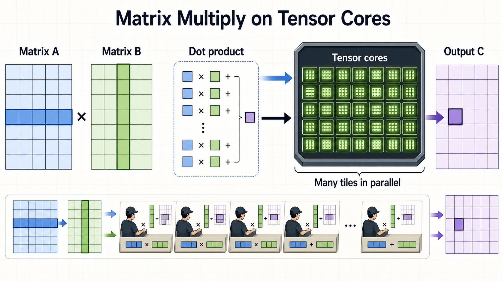
The number of arithmetic operations performed for each byte moved across a named memory boundary. A value is high or low only relative to a particular machine and memory level. Source.
Attention

A neural-network calculation that lets a token draw different amounts of information from selected token positions. During ordinary text generation, a token may use itself and earlier tokens but not later ones. Source.
Attention head
One parallel set of learned calculations that creates query, key, and value vectors and performs attention with them. A layer can run several heads so it can learn different comparison patterns, then combine their outputs. Source.
Autoregressive generation
Generating a sequence one accepted item at a time, with each new item depending on the items already accepted. Ordinary language-model decoding generates tokens this way. Source.
Backpropagation and backward pass
Backpropagation applies the chain rule backward through a neural network to calculate how the loss changes with each parameter. The computation that performs this work is commonly called the backward pass; an optimizer later uses the resulting gradients to update the parameters. Source.
Bandwidth and memory bandwidth
Bandwidth is a maximum or measured data-transfer rate over a stated connection. Memory bandwidth is the rate between a processor and a named level of memory; every figure should say whether it is theoretical or measured and which directions or operations it includes. Source.
Batch and batching
A batch is a group of examples or active requests processed together. Batching can reuse data and raise total throughput, but larger batches also use more memory and can make an individual request wait. Source.
Benchmark
A controlled test used to compare performance under stated conditions. A useful benchmark names the workload, hardware, software, numerical format, input and output sizes, number of simultaneous requests, and measurement rules. Source.
Bfloat16 (BF16)
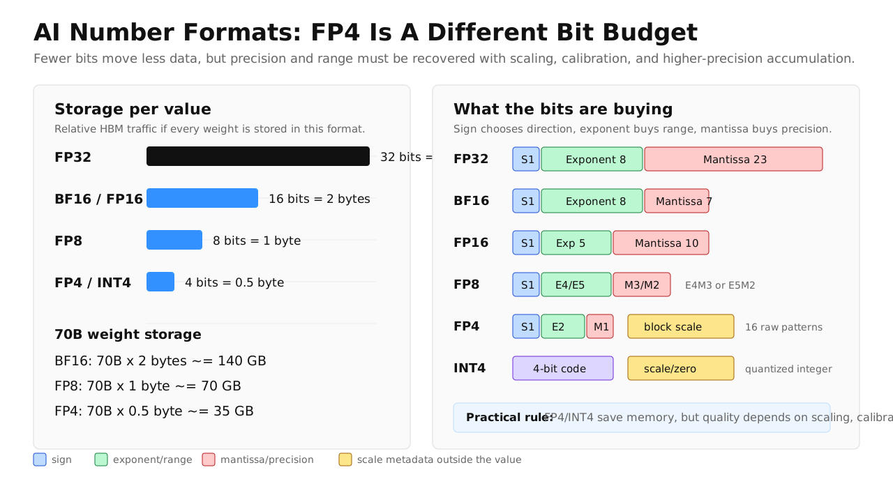
Bfloat16 is a 16-bit floating-point format. It covers roughly the same range of magnitudes as 32-bit floating point but records fewer fine distinctions between nearby values. Source.
Binning

Testing manufactured chips and sorting them into product grades according to the specifications they meet, such as working features, frequency, or power. A lower bin is not necessarily a defective chip. Source.
Bit and byte
A bit represents one of two values, conventionally zero or one. A byte contains eight bits; in decimal units, one gigabyte is one billion bytes. Source.
Cache
Storage that keeps copies of data near a consumer so a later access may avoid a slower source. A cache helps only when it contains the needed data. Source.
Memory capacity
The amount of data a memory system can hold. Memory capacity answers whether the required weights and working data fit; it does not say how quickly they can be read. Source.
Checkpoint
A saved collection of model or training state. It may be a released model or a recovery snapshot used to resume a run; it may also be split across files or machines. This meaning is different from activation checkpointing, which reduces temporary memory during one calculation. Source.
Chiplet
A die designed to be combined with other dies in one package. Chiplets may divide one function or provide different functions and do not have to be physically tiny. Source.
Cluster
.jpg)
A group of connected computers that work together on a shared task or service. Calling a system a cluster does not by itself specify its connection speed, size, or reliability. Source.
Compute-bound
A condition in which available arithmetic throughput is the main performance limit for a specified program and machine. Memory traffic, communication, or dependencies may be separate limits in another implementation. Source.
Model context
The information represented in the input supplied for the current model calculation. A service may build the model context from instructions, messages, retrieved material, and tool results; information outside that supplied input is not automatically available to the model. Source.
CPU
Central processing unit: a general-purpose processor that runs operating systems and a wide variety of programs. CPUs can perform parallel work, but high-performance cores also devote substantial hardware to reducing delay on irregular and decision-heavy code. Source.
Customer qualification
Testing and approval by a customer that a component meets the customer's platform and reliability requirements before broader use. Passing a supplier's internal tests does not automatically complete a customer's qualification process. Source.
Data parallelism
A training method in which workers process different examples and combine their gradients or updates. The model parameters may be copied on each worker or divided by a sharded variant. Source.
Decode
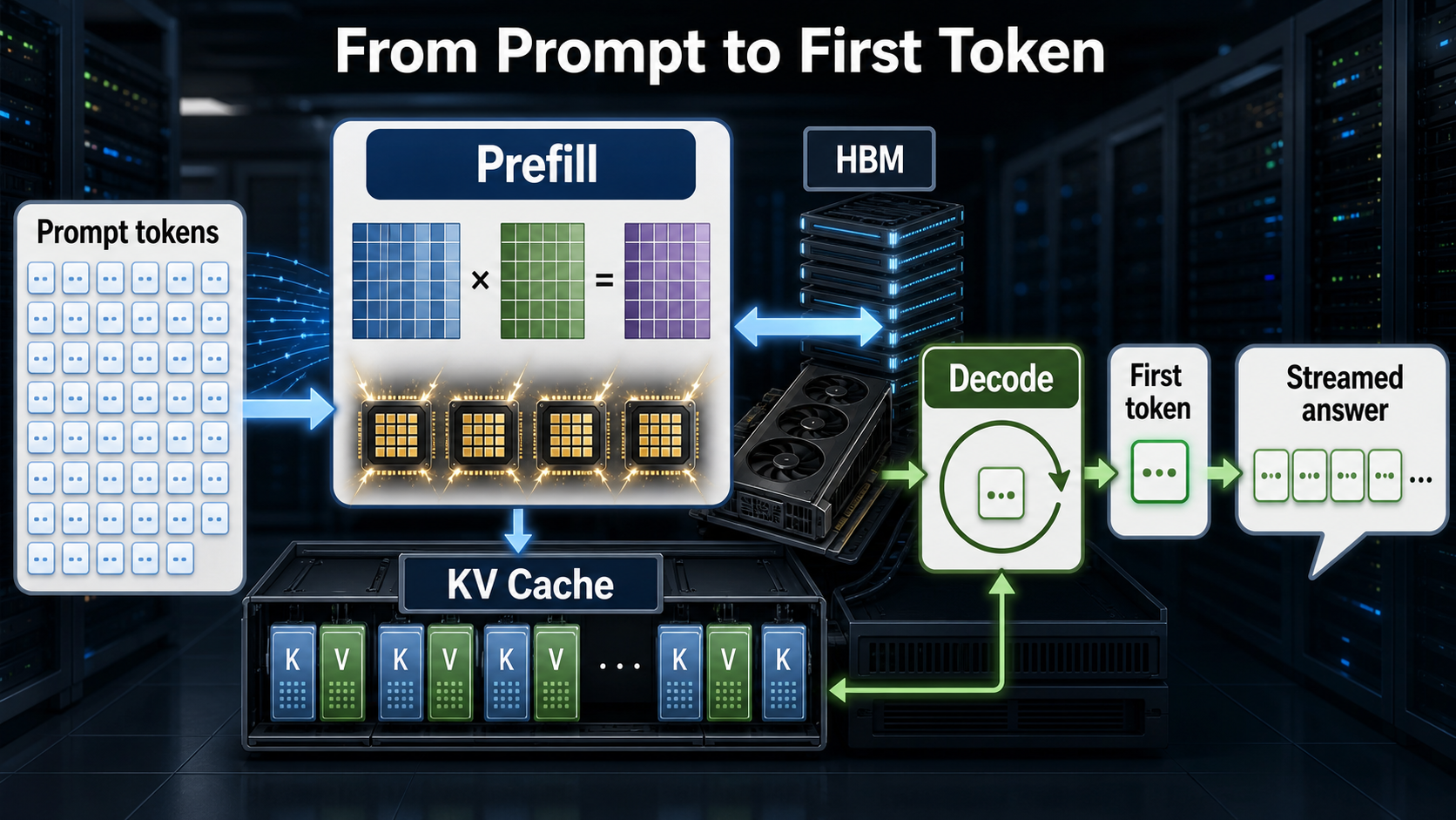
In autoregressive language-model serving, the phase that generates output tokens after the prompt has been processed. Accepted output tokens are produced in sequence, although an implementation may test several candidates at once. Source.
Die
One piece of semiconductor material containing a fabricated circuit. A die is cut from a processed wafer and may later be combined with other dies inside a package. Source.
DRAM
Dynamic random-access memory: memory that stores each bit in a cell whose charge must be refreshed. GDDR and HBM are DRAM families; DRAM is denser but generally slower than the on-chip SRAM used for small memories. Source.
Embedding
A learned vector representation of an item. In this course, a token embedding is the learned list of numbers selected by a token identifier before transformer layers add context to that representation. Source.
Ethernet
A standardized family of wired network technologies used from local networks to data centers. A quoted Ethernet rate is a link rate; packet and protocol overhead can make useful application throughput lower. Source.
Floating-point
A way to encode numbers using a sign, a scale called an exponent, and significant digits. Different floating-point formats trade storage and precision against the range of magnitudes they can represent. Source.
Feed-forward block
The part of a transformer layer that applies the same learned neural-network calculation separately to each token position after attention has exchanged information among positions. Transformer designs vary in the exact calculation they use. Source.
Floating-point operation (FLOP)
A floating-point operation, or FLOP, is one counted arithmetic operation under a stated convention; a fused multiply-and-add is commonly counted as two. FLOP/s is a rate, and it is incomplete unless the number format, operation, and any sparsity assumption are stated. Source.
Forward pass
The computation from a model's input through its prediction and, during training, its loss. Training retains or later recreates selected intermediate results so the backward pass can calculate gradients. Source.
Foundry
A semiconductor manufacturer that fabricates circuits, often from designs supplied by other companies. A pure-play foundry primarily manufactures customer designs rather than selling its own chip designs. Source.
FP8
A family of one-byte floating-point formats that divide their bits differently between numerical range and fine detail. A claim using FP8 must name the exact format, operation, and accumulation method. Source.
32-bit floating point (FP32)
The common name for the standardized 32-bit binary floating-point format. Each value uses four bytes and records more numerical detail than BF16, but more precision does not guarantee a better or faster model result. Source.
GDDR
Graphics Double Data Rate: a family of high-data-rate DRAM used for graphics and some AI systems. Its capacity and bandwidth depend on the generation and system design. Source.
GPU

Graphics processing unit: a processor architecture developed for graphics and organized for high-throughput parallel work. Many neural-network operations suit its matrix and vector hardware, but performance still depends on software and data movement. Source.
Gradient
Numbers showing how small changes to the parameters would change the training loss. An optimizer uses gradients to calculate an update; a gradient is not the update itself. Source.
HBM
High Bandwidth Memory: stacked DRAM with a very wide connection, commonly placed in the same package as a high-end accelerator. HBM raises bandwidth but adds demanding memory-stacking, packaging, and testing work. Source.
Inference
Using a trained model to calculate an output from new input without performing an ordinary training update to its parameters. Output may be text, a prediction, an image, an embedding, or another model result. Source.
InfiniBand

A switched network design built for high data-transfer rates and short delays. It is widely used in high-performance-computing and AI clusters and can move data directly between computers' memory with little work from their CPUs. Source.
Accelerator interconnect
A connection that carries data among nearby accelerators in a tightly coupled system. Its bandwidth, delay, connection map, and software support affect how well work can be split across chips. Source.
Interposer

An intermediate wiring structure that creates dense connections among dies inside a package. Interposers can be built in different ways, and not every HBM package uses the same kind. Source.
Inter-token latency
The elapsed time between two generated output tokens. It differs from time to first token and from an average time-per-token measure calculated over a whole response. Source.
Kernel
.PNG)
A small program that a GPU runs across many parallel workers. The word has other meanings in operating systems, so this course uses it only in the GPU sense. Source.
Kernel fusion
Combining compatible calculations into one GPU kernel so a temporary result can stay on the chip or be eliminated instead of being written to large device memory and read back. Fusion can use more on-chip resources and is not always faster. Source.
Key-value cache (KV cache)
The key and value arrays already computed by each attention layer for earlier tokens. Reusing them during decode avoids recomputing those earlier keys and values, but the cache consumes more memory as the retained sequence grows. Source.
Latency
The elapsed time from the start of an operation or request to a stated completion point. A latency figure is incomplete unless it says exactly what starts and ends the measurement. Source.
Latency hiding
Keeping other work ready so a processor can run it while one group waits for data or an earlier operation. This reduces idle time but does not make the underlying delay disappear. Source.
Model layer
One stage of a neural network that transforms input values into output values using learned parameters and other operations. Modern models usually apply many model layers in sequence. Source.
Large language model
A language model with a very large number of learned parameters. “Large” has no universal numerical threshold. Source.
Lithography
A chip-manufacturing process that uses light and a patterned mask to define features in a light-sensitive coating on a wafer. Deposition, etching, and other steps then build the physical structures. Source.
Training loss
A numerical score for a model's error on an example or batch. Training calculates gradients of the loss and uses them to guide parameter updates. Source.
Matrix and matrix multiplication
A matrix is a rectangular array of numbers. Matrix multiplication combines rows from one matrix with columns from another to produce a new matrix; many neural-network layers spend much of their arithmetic on this operation. Source.
Memory-bound and memory-bandwidth-bound
A condition in which moving data through a named memory connection is the main performance limit for a specified program and machine. Changing the batch, software, or hardware can change whether the same operation is memory-bound. Source.
Memory wall
The growing mismatch between how quickly processors can perform arithmetic and how quickly memory systems can supply data. Caches, data reuse, lower precision, and wider memory connections address parts of this problem. Source.
Mixed-precision training
Training that uses more than one numerical format, choosing each according to the operation and numerical need. A common pattern uses compact values for much of the arithmetic and more precise values for selected updates or accumulated results. Source.
AI model
A learned system of calculations that maps an input to a prediction or other output. Training adjusts an AI model's parameters; inference uses a trained model to produce outputs. Source.
Moore's law
An industry observation that the number of components economically placed on an integrated circuit tended to grow rapidly over time. It is not a physical law and does not promise that every program becomes faster at the same rate. Source.
Neural network
A model built from connected layers whose behavior depends on learned parameters. “Neural” is historical terminology; the model is a mathematical computation, not a biological brain. Source.
Number format
The rule that says how a pattern of bits represents a number. Formats differ in storage size, range, precision, and the operations that hardware supports. Source.
Optimizer
A training algorithm that uses gradients and an update rule to change model parameters. Some optimizers, including Adam, keep extra state from earlier steps. Source.
Package
The structure that protects one or more dies and connects them to the rest of a system. Some accelerator packages also include nearby HBM, but memory is not part of every chip package. Source.
Parameter
A numerical value adjusted by training, commonly a weight or bias. Parameter count describes how many learned values a model has but does not by itself determine quality, file size, or active computation. Source.
Pipeline parallelism
A method that assigns sequential groups of model layers to different devices. Intermediate results move forward through the stages, while training gradients move backward; idle gaps and unequal stage times reduce efficiency. Source.
Electrical power and electrical energy
Electrical power is the rate of energy use and is measured in watts; one watt equals one joule per second. Electrical energy is power accumulated over time, so one kilowatt used for one hour equals one kilowatt-hour. Source.
Precision
How finely a numerical representation distinguishes nearby values. Precision is different from range, which describes the smallest and largest magnitudes the format can represent. Source.
Direct preference optimization
A post-training method that learns from comparisons between preferred and less-preferred responses without first fitting a separate reward model. It is different from reinforcement learning from human feedback. Source.
Prefill
The language-model inference phase that processes the supplied input tokens and prepares the initial KV cache before output-token generation. Time to first token also includes possible network, queue, tokenization, and scheduling delay. Source.
Process node

A foundry's name for a generation of transistor and wiring technology. Modern labels such as “3 nanometer” do not measure one physical feature and cannot be compared directly across foundries. Source.
Prompt
Input supplied to a generative model for one call. A service may combine user content with instructions, earlier messages, retrieved material, and tool results before constructing the model's input. Source.
Quantization
Mapping values from a larger set into a smaller set of representable values, often for model weights or intermediate results. It can reduce storage and memory traffic, but speed and quality effects depend on the method, model, and hardware. Source.
Query-key-value (QKV)
Three numerical roles in attention. A query is compared with keys to obtain match weights; those weights determine how the corresponding values are mixed into the attention output. Learned calculations create Q, K, and V from the current token representations; they are not human-written labels. Source.
Register
A tiny storage location used directly by processor instructions for values needed immediately. Registers are much smaller and closer to arithmetic hardware than device memory. Source.
Reinforcement learning
A family of methods in which an agent learns what actions to take so as to increase expected cumulative reward. Human preferences can provide a reward signal in one application, but they are not part of the general definition. Source.
Reticle limit
Informal shorthand for the maximum rectangular field a lithography scanner exposes at once. It constrains the size of a conventional die made with one exposure field. Source.
Roofline model
A performance bound that compares a machine's peak arithmetic rate with its memory bandwidth multiplied by arithmetic intensity. The lower of those two ceilings limits the attainable arithmetic rate in the simplified model. Source.
Scale-out
Connecting multiple servers or tightly connected accelerator groups through a broader network. Scale-out describes system organization, not a guarantee about distance, speed, or network design. Source.
Scale-up
Connecting processors within a tightly coupled group using links designed for high bandwidth and low latency. The group may be inside a server or extend across a rack; the term describes system organization rather than distance alone. Source.
GPU scheduler
Control hardware that chooses which ready group of GPU work runs next. It can issue another ready group while one group waits for data. Source.
Sharding
Dividing specified model data or training state across workers so each holds only a share. It lowers the memory needed on one worker but creates communication when another worker needs a piece. Source.
SRAM
Static random-access memory: fast memory technology used for small on-chip caches and working memories. It uses more chip area per stored bit than DRAM, so processors include much less of it. Source.
Structured sparsity
A pattern in which zeros appear in the exact arrangement that supported hardware can skip. Arbitrary zeros do not automatically qualify a calculation for an advertised sparse rate. Source.
Supervised fine-tuning
Additional training on examples that pair an input with a desired output. It can teach a pretrained model a task or response style without defining every later post-training method. Source.
Tensor core
NVIDIA's name for specialized GPU units that perform supported matrix multiply-and-accumulate operations. Their advertised rate depends on the numerical format and may also assume a supported sparsity pattern. Source.
Tensor parallelism
A method that splits operations inside a model layer, commonly a matrix multiplication, across devices. The devices must exchange partial results frequently, so connection performance matters. Source.
Tile
A small rectangular block cut from a larger array of numbers. GPU programs move and reuse tiles in nearby memory so many calculations can share the same loaded data. Source.
Throughput
The amount of completed work per unit time, such as requests or output tokens per second. It differs from latency, the time one specified request takes; batching can raise throughput while increasing waiting. Source.
Time to first token
The elapsed time from submitting a request until its first generated output token arrives. Depending on the measurement boundary, it may include network transfer, queueing, tokenization, scheduling, and prompt processing. Source.
Token
An identifier produced by a model's tokenizer, representing a whole word, part of a word, punctuation, or another text fragment. Token-to-word ratios vary with language, text, model, and tokenizer. Source.
Tokenization and tokenizer
A tokenizer applies a fixed vocabulary and splitting rules to map input into token identifiers; tokenization is that conversion process. Different model families can split the same text differently. Source.
Tool call
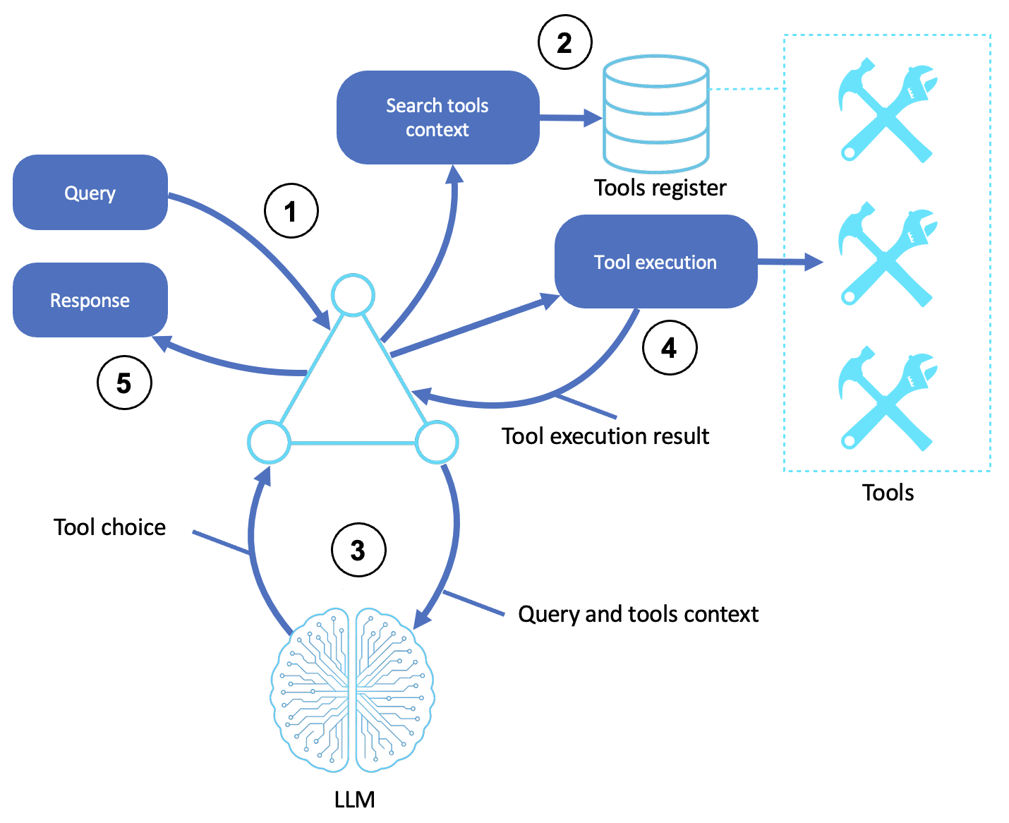
A structured request from a model asking ordinary software to run a named external function with specified inputs. The surrounding application—not the model—must validate permissions, execute the function, and return its result. Source.
Topology
The pattern of connections among processors, servers, and switches. Together with link rates, routing, and software, topology affects available paths, congestion, delay, and failure behavior. Source.
Training
Adjusting a model's parameters using data so that a stated error or reward measure improves. Neural-network training commonly uses a training loss, backpropagation, and an optimizer; only large runs require many machines. Source.
Transformer
A neural-network design introduced in 2017 that arranges attention and other calculations in repeated blocks. Most current large language models use transformer-based designs, with many variations. Source.
Transistor
A semiconductor device that can switch or control an electrical signal. Modern processors combine many transistors to build arithmetic, memory, and control circuits. Source.
Wafer
A circular slice of semiconductor material on which a factory builds many copies of a circuit. The processed wafer is tested and cut into individual dies. Source.
Weight
A learned parameter that a model multiplies by another value; many weights are entries in matrices. Not every parameter is a weight. Source.
Vector
An ordered one-dimensional list of numbers. A token embedding and each query, key, or value inside one attention head are vectors; the number of entries depends on the model design. Source.
Vocabulary
The set of token pieces and identifiers available to a tokenizer and its model. The tokenizer maps input text to identifiers from this set, and a text-generating model assigns an output score to each allowed vocabulary token. Source.
Die yield
The share of manufactured dies that meet the required tests. Die yield depends on the design, defect rate, process, and test criteria; it is not the same as binning acceptable parts into product grades. Source.